Getting Started

Get started by completing the total energy tutorial.

Input files

NanoDCAL+ reads input files in the JSON format. The JSON format is lightweight, portable and essentially composed of Python’s basic types like: dict, list, int, float, str. It is thus convenient to prepare, read or write input files in Python using the JSON module. NanoDCAL+ accepts so-called exhaustive input files, which contain almost all of a simulation parameters, including:

• atomic orbital basis functions (if any)

• geometry

• pseudopotentials

• solver parameters

• etc.

Such files are convenient to keep as reference input, since they are not susceptible to changes in default parameters between version, among other advantages. But it is impractical to produce them from manually. Which is why NanoDCAL+ works in tandem with nanotools, a Python interface which makes it convenient to create structures, write input files and read the output files produced by NanoDCAL+.

System and calculator classes

Atomic systems are described by the System class. System objects can be initialized from an Atoms and a Cell object (or their corresponding dictionaries). System objects have additional attributes (such as Kpoint) which are described here. nanotools includes various calculator classes like the basic (and most important) TotalEnergy class. A TotalEnergy instance holds all the data regarding a given calculation:

• the system description and simulation parameters;

• the solvers’ parameters;

• the output data.

A TotalEnergy object can be initialized from a System object or a corresponding dictionary or JSON file. All parameters are initialized during its creation, while retaining values specified in the seed objects or dictionary. The resulting object then maps to an exhaustive input file required by NanoDCAL+. It contains additional methods which may provide valuable information about the system (e.g. number of atoms, converting units). The structure is easily deduced from the API documentation.

A typical input file (here GaAs-FCC) looks as follows:

Listing 1 Input file for a GaAs crystal

from nanotools import Atoms, Cell, Kpoint, System, TotalEnergy
a = 2.818
cell = Cell(avec=[[0.,a,a],[a,0.,a],[a,a,0.]], resolution=0.12)
fxyz = [[0.00,0.00,0.00],[0.25,0.25,0.25]]
atoms = Atoms(fractional_positions=fxyz, formula="GaAs")
sys = System(cell=cell, atoms=atoms)
calc = TotalEnergy(sys)
calc.solve()
print(calc.energy.etot)

Atomic configurations

Atomic configurations consist in sets of coordinates and species. The coordinates are specified either by the positions or fractional_positions attribute of Atoms objects. The atomic species are specified in the attribute formula of an Atoms object. Each atom has a position and a corresponding label or symbol, and each label corresponds to a species. In supercells, one can use the following short hand instead of repeating symbols.

formula="GaGaGaGaGaGaGaGaGaGaGaGaGaGaGaGaAsAsAsAsAsAsAsAsAsAsAsAsAsAsAsAs"

is equivalent to

formula="Ga(16)As(16)"

For larger systems, one can simply specify the configuration in an xyz-file and pass it to either the positions or fractional_positions attribute. In this case formula need not be set.

Pseudopotentials

nanotools can read pseudopotential (PS) files and numerical atomic orbital (NAO) basis files generated by our atomic code Nanobase, i.e. the same PS/NAO files as those with NanoDCAL and RESCU distributions. To install PS, untar the PS archive provided to you with the source code in a known folder and set the environment variable NANODCALPLUS_PSEUDO to that folder. Note that you may need to change this depending on your applications: when using LDA you may set NANODCALPLUS_PSEUDO=path/to/lda/pseudos; when using PBE you may set NANODCALPLUS_PSEUDO=path/to/pbe/pseudos. Or simply copy the PS files you will use to $PWD and set NANODCALPLUS_PSEUDO=$PWD.

The DFT package RESCU+ and the NEGF-DFT package NanoDCAL+ are pseudopotential (PS) codes. They support the Troullier-Martin (TM) PS and the Optimized Norm-Conserving Vanderbilt (ONCV) PS.

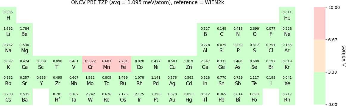
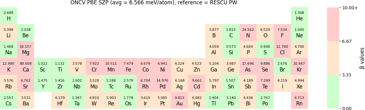
Both RESCU+ and NanoDCAL+ use numerical atomic orbital (NAO) functions to form linear combination of atomic orbital basis (LCAO). These NAOs have been carefully tested using two methods. The first is the standard Δ-gauge which quantifies the difference of the equation of state (EOS) calculated by RESCU+ using LCAO basis and two benchmarks. One set of benchmark results was from the full potential WIEN2k package; while the second set of benchmark results was from the plane waves (PW) method of RESCU. Typically, Δ-values below 2 meV/atom suggests the LCAO basis to be excellent while somewhat higher values are also quite acceptable for many applications. The second test of the NAO is via a β-gauge that quantifies the difference of electronic band structures obtained by RESCU+ using LCAO basis and benchmark results, where the benchmarks were obtained from RESCU using the PW basis. The β-values have the same order of magnitude and unit as Δ, and a small β implies small deviation of band structures between LCAO and PW basis. In NEGF-DFT quantum transport simulations using NanoDCAL+ and/or many other applications, accurate band structures are critical.

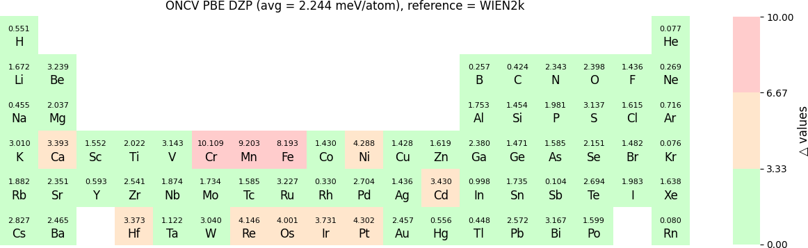
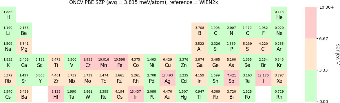
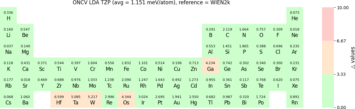
In release 2023B, for ONCV, Triple Zeta Polarization (TZP), Double Zeta Polarization (DZP) and Single Zeta Polarization (SZP) NAO basis functions are provided. TZP is the largest basis followed by DZP and SZP. The Δ-values for TZP, DZP and SZP basis with respect to the WIEN2k benchmark using GGA-PBE, are shown in the following three periodic tables:

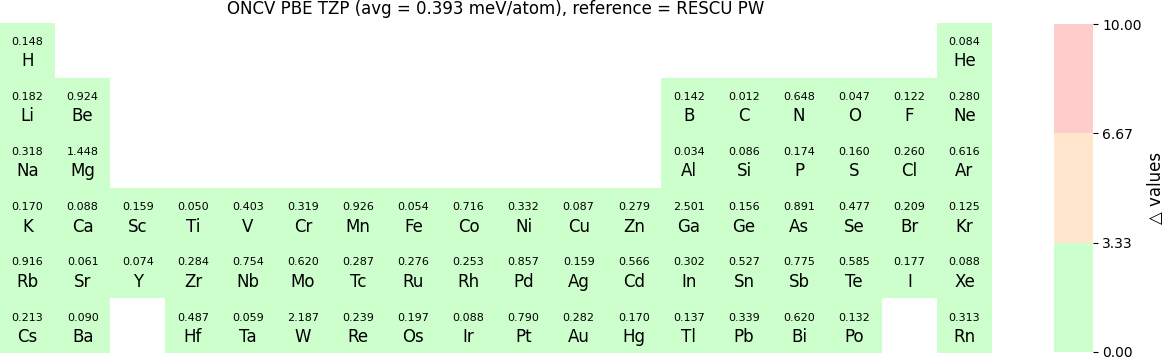
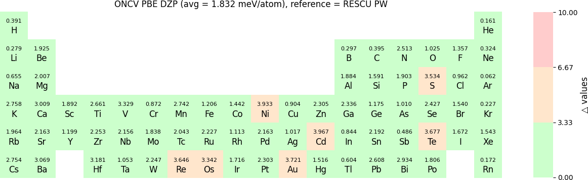
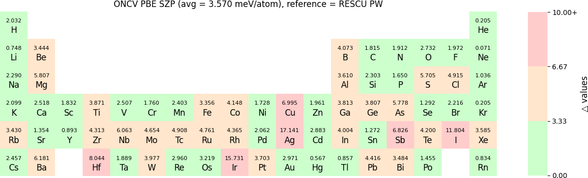
The Δ-values for the above NAO functions benchmarked with RESCU using PW basis are shown in the following three periodic tables:

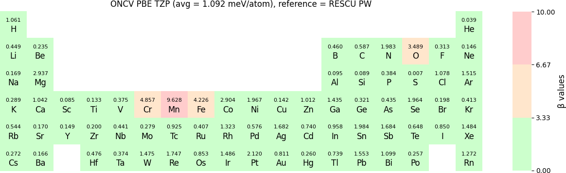
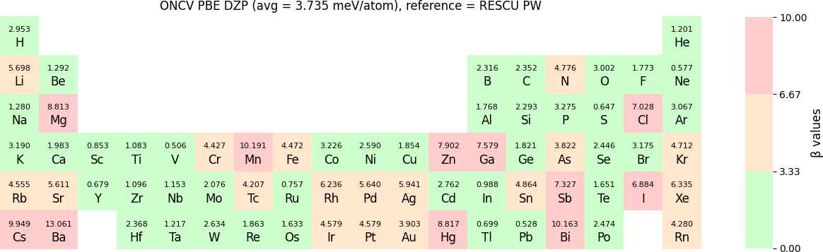
The β-values for the TZP, DZP and SZP NAO functions benchmarked with RESCU using PW basis, are shown in the following three periodic tables.

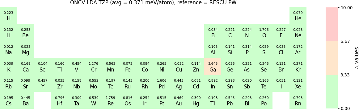
In release 2023B, TZP basis functions generated by the LDA exchange-correlation functional are also provided. Their Δ values benchmarked with WIEN2k and with RESCU using PW basis, are shown in the following two periodic tables:

\(\Delta\) values for TZP basis sets with respect to the PW method (LDA):

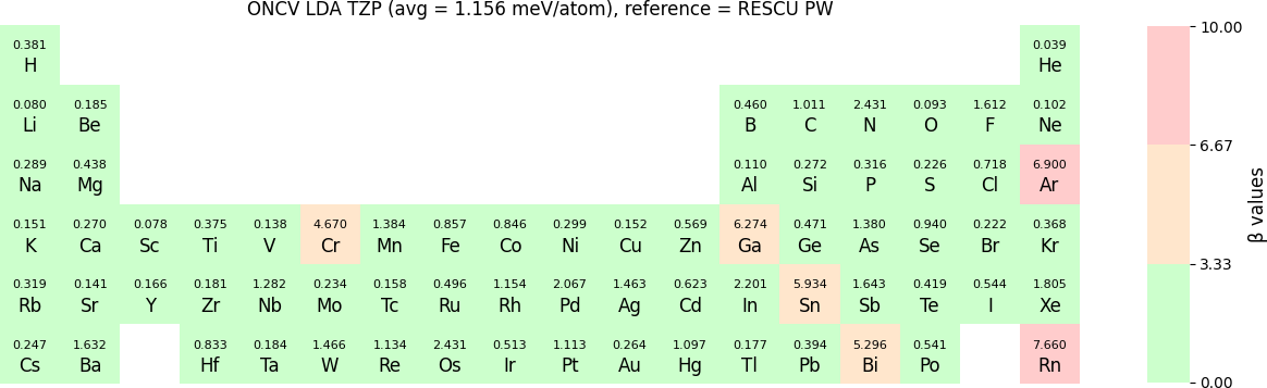
The β values for TZP basis sets with LDA benchmarked by RESCU using PW basis are shown in the following periodic table:

The following table provides a summary of the two metrics Δ and β in units of meV/atom for four NAO databases using ONCV PS. These databases were optimized using different exchange-correlation functionals and come in various sizes, including TZP, DZP and SZP. Δ (LCAO-WIEN2k) represents Δ values of the LCAO basis sets benchmarked with WIEN2k, Δ (LCAO-PW) represents Δ values benchmarked with RESCU using PW basis, and β (LCAO-PW) represents the β values between LCAO and PW basis. Mean values, averaged over 70 elements in the periodic table, of the two metrics and the corresponding standard deviations (SD) are provided for statistical purposes.

metric	Δ (LCAO-WIEN2k)		Δ (LCAO-PW)		β (LCAO-PW)
statistics	mean	SD	mean	SD	mean	SD
ONCV PBE TZP	1.0947	1.6716	0.3933	0.4451	1.0924	1.4246
ONCV PBE DZP	2.2439	1.8502	1.8317	1.0409	3.7351	2.8003
ONCV PBE SZP	3.8149	3.2230	3.5696	3.0109	6.5664	10.026
ONCV LDA TZP	1.1513	1.3435	0.3706	0.5464	1.1560	1.6726

While it is the responsibility of users to select the most proper LCAO basis for their applications, here are some general suggestions:

1. Experimenting the size of the basis sets (TZP, DZP or SZP) according to your system and goal. Larger basis sets may give more accurate results at the expense of computational time. Smaller basis sets can also give quite reasonable results for many applications. DZP basis sets are suggested for a balance between accuracy and computational cost.

2. Always test convergence before performing lengthy production calculations, by gradually increasing the real space grid, which corresponds to the mesh cut-off energy.

3. For stress tensor calculations of magnetic materials, fine real space grids should be tested (for example, 0.06 Bohr grid spacing for Fe, Co, Ni etc.) to attain precision.

Arrays

Many quantities are conveniently represented as arrays. For example, lattice vectors are written as

avec = [[1.,2.,3.],[4.,5.,6.],[7.,8.,9.]]

If arrays with more than one dimension are written as vectors, they will be reshaped automatically. We strongly suggest to explicitly specify the multidimensional array as above. If for some reason you need to employ one-dimensional arrays, read the following. NanoDCAL+ uses the so-called Fortran order, which means that a vector is reshaped filling the 1st dimension, then the 2nd, then the 3rd etc. This means that

avec = [1.,2.,3.,4.,5.,6.,7.,8.,9.]

is reshaped to

avec = [[1.,4.,7.],[2.,5.,8.],[3.,6.,9.]]

which corresponds to a matrix

\[\begin{split}\begin{pmatrix} 1 & 4 & 7\\ 2 & 5 & 8\\ 3 & 6 & 9\\ \end{pmatrix}\end{split}\]

By contrast, there exist the so-called C ordering where multidimensional arrays are filled backward, i.e. starting by the last dimension.

This means that

avec = [1.,2.,3.,4.,5.,6.,7.,8.,9.]

is reshaped to

avec = [[1.,2.,3.],[4.,5.,6.],[7.,8.,9.]]

which corresponds to a matrix

\[\begin{split}\begin{pmatrix} 1 & 2 & 3\\ 4 & 5 & 6\\ 7 & 8 & 9\\ \end{pmatrix}\end{split}\]

Units

NanoDCAL+ uses the Python library Pint to keep track of units. What you need to know to get started is that

• Quantities with units in NanoDCAL+ are Quantity instances.

• You can get the magnitude of a Quantity object a with a.m.

• You can get the unit of a Quantity object a with a.u.

• You can import the unit registry from nanotools.utils, would you like to create Quantity objects of your own.

You may refer to the Pint documentation if you would like to know more about the library’s functionalities.

NanoDCAL+ works with two unit systems:

• extended SI: eV and \mathring{\text{A}}

• atomic: hartree and bohr

The units of the exhaustive input file are hartree and bohr by default, since these files are intended for internal use of the Fortran code. Python entities, like a seed dictionary or any data in a TotalEnergy object, are in SI by default. Attributes which are of the Quantity class are automatically converted on entry. One can specify units in two ways:

• use the unit registry from nanotools.utils.

• pass a two-element tuple containing the magnitude and the unit as a string.

For example, in Listing 1, I can specify the units of avec as follows

from nanotools.utils import Quantity, ureg
a = 2.818
cell = Cell(avec=[[0.,a,a],[a,0.,a],[a,a,0.]] * ureg.angstrom, resolution=(0.2, "bohr"))
# [...]
print(calc.energy.etot.to("picojoules"))

First, avec is converted to a Quantity with units of angstrom multiplying by ureg.angstrom. Then, resolution is specified in bohr, passing a tuple consisting of a float and the string bohr.

Return switches

To save time, a user may set return switches to perform or skip certain calculations. For example the atomic forces, obtained upon completing a ground state calculation, are not always necessary. It is thus possible to set ["energy"]["forces_return"], which corresponds to ["energy"]["forces"], to false and save time by skipping the force calculation. Similarly, several output parameters have a corresponding _return parameter.