7. Charge noise in quantum dots
7.1. Requirements
7.1.1. Software components
QTCAD
7.1.2. Mesh file
qtcad/examples/practical_application/meshes/gated_dot.msh2
7.1.3. Python script
qtcad/examples/practical_application/7-noise.py
7.1.4. References
7.2. Briefing
In the previous tutorial, we have investigated the dynamics of a qubit subject to electric dipole spin resonance. We started out by considering Rabi oscillations within the subspace of the two lowest-energy eigenstates. We then went beyond this approximation by considering leakage into higher-energy states. In this tutorial, we will consider another nonideality to which a qubit may be subject to: charge noise.
Specifically, in Electric dipole spin resonance and Rabi oscillations, the Hamiltonian was given by
where \(\hat H_0\) is the qubit Hamiltonian and \(\delta \hat V\) is the Hamiltonian describing the amplitude of the perturbation produced by the time-dependent electric field (the frequency of which is given by \(\omega\)).
Instead, in this tutorial, we will aim to simulate the dynamics assuming the Hamiltonian
where \(\beta(t)\) is a stationary and ergodic Gaussian random process with vanishing mean—it represents charge noise on the gate driving the qubit. More theoretical background on noisy EDSR is given in the subsection called A more realistic scenario: noisy electric-dipole spin resonance in the Quantum control theory section.
7.3. System initialization
We start by importing relevant modules.
import numpy as np
import pathlib
from matplotlib import pyplot as plt
from device import constants as ct

import qutip
from qubit import spectra, dynamics, noise
All these modules were previously seen, except from noise, which is used to
model two-level systems subject to noise.
The system and drive Hamiltonians are then loaded from the results of Electric dipole spin resonance and Rabi oscillations and defined in units where \(\hbar=1\) (as required by QuTiP).
# Paths to system and drive Hamiltonians
script_dir = pathlib.Path(__file__).parent.resolve()
path_h0 = str(script_dir/'output'/'h0.npy')
path_u = str(script_dir/'output'/'u.npy')

# Load system and drive Hamiltonians and rewrite in units of hbar = 1
H0 = np.load(path_h0)/ct.hbar
delta_V = np.load(path_u)/ct.hbar
Several timescales are relevant for the simulation that we will perform. These timescales include the inverse of the qubit frequency (i.e., the difference between the two spin-qubit eigenenergies) and the Rabi period.
# Define relevant frequencies and time scales of the problem
omega = H0[0,0] - H0[1,1] # qubit frequency
omega_Rabi = np.absolute(delta_V[0,1]) # Rabi frequency on resonance
T_Rabi = 2*np.pi/omega_Rabi # Rabi period
We also need to define a time array on which we will sample the system and noise dynamics.
# Define time array
T = 20 * T_Rabi # Total time of the simulations
times = np.linspace(0, T, 1000) # Times at which dynamics are simulated.
Finally, we initialize a Dynamics object and a Noise object, which will
be used later.
# Initialize objects that will handle dynamics and noise.
dyn = dynamics.Dynamics()
N = noise.Noise()
7.4. Simulation without noise
To model the dynamics of our system without noise, we use a procedure similar
as in the previous tutorial. To simplify the treatment, we will employ the
H_RF method of the dyn object, which returns a QuTiP Qobj corresponding
to the Hamiltonian \(\hat H(t)=\hat H_0 + \delta \hat V \cos (\omega t)\).
# Simple simulation without noise
# The Hamiltonian H = H0 + delta_V cos(omega*t) in a frame rotating
# at frequency omega.
H = dyn.H_RF(H0, delta_V, omega)
The system dynamics can then be solved as before.
# Solve for the dynamics without any noise.
psi0 = qutip.basis(2, 0) # initial state
result0 = qutip.mesolve(H, psi0, times)
Next, we compute and plot the expectation values of Pauli operators,
\(\braket{\sigma_z(t)}\) and \(\braket{\sigma_y(t)}\) using
the qutip.expect function.
# Plot expectation values of sigma_z and sigma_y as a function of time.
fig, axes = plt.subplots(2)
fig.set_size_inches((8,8))
#<sigma_z (t)>
axes[0].plot(result0.times, qutip.expect(qutip.sigmaz(), result0.states))
#<sigma_y (t)>
axes[1].plot(result0.times, qutip.expect(qutip.sigmay(), result0.states))
# Labels
axes[0].set_ylabel(f'$\left< \sigma_z (t) \\right>$', fontsize=20)
axes[1].set_ylabel(f'$\left< \sigma_y (t) \\right>$', fontsize=20)
axes[0].set_xlabel(f'$t \, (s)$', fontsize=20)
axes[1].set_xlabel(f'$t \, (s)$', fontsize=20)
plt.show()
This should result in the following figure.
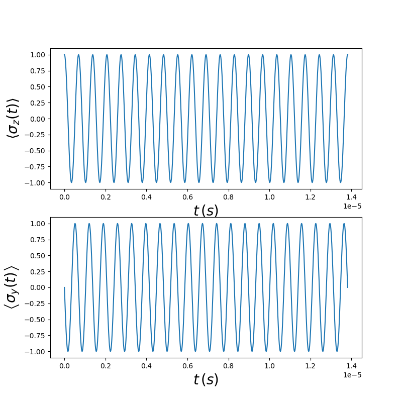
Fig. 7.4.4 Expectation values of Pauli operators ignoring charge noise
7.5. Simulation with noise
7.5.1. Modeling the charge noise
Following the procedure described in Electric dipole spin resonance—Noise, to generate a
stationary, Gaussian, and ergodic random process with vanishing mean
\(\beta(t)\), we start by defining a spectral density for the noise.
For this purpose, we take this spectral density to be a Lorentzian centered
at angular frequency w0 = 0 with width equal to the Rabi frequency,
which we have previously stored as omega_Rabi. Furthermore, we define
a sampling frequency (or frequency resolution) for the discrete implementation
of this spectral density in such a way that its inverse, T0 is much greater
than all other timescales of the problem. Finally, we define the total
power of this noise, S0. With these elements, we can define the Lorentzian
spectral density using the spectra.lorentz method.
# Include charge noise which is assumed to affect only the gate which
# generates the drive delta_V.
# Lorentzian spectrum
S0 = 0.01 # Total power
wc = omega_Rabi # Cutoff frequency
w0 = 0 # Central frequency
# T0 should be much larger than the largest time scale of the problem under consideration.
# Used to properly define the Fourier series of the time series related to the noise.
T0 = 50 * T_Rabi  # Must take T0 such that 2*pi/T0 << wc to resolve the spectrum
omega_max = 5*wc
wk = np.arange(0, omega_max , 2*np.pi/T0) + w0
spectrum = spectra.lorentz(wk, S0, wc, w0 = w0)
This Lorentzian can then be plotted as follows.
# Plot spectrum
fig, axes = plt.subplots(1)
fig.set_size_inches((10,6))
axes.plot(wk, spectrum)
axes.set_ylabel(f'$S_\\beta(\omega) \, (s)$', fontsize=20)
axes.set_xlabel('$\omega \, (s^{-1})$', fontsize=20)
axes.set_title('Lorentzian spectral density', fontsize=30)
plt.show()
This should result in the following figure.
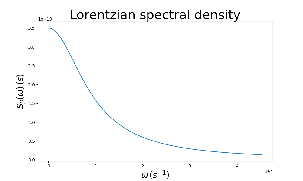
Fig. 7.5.10 Lorentzian spectral density for the charge noise
Having obtained the spectral density, a time series for the charge noise can be
randomly generated using the N.gen_process method.
# Plot time series for the charge noise affecting the gate responsible for
# delta_V.
beta = N.gen_process(times, spectrum, wk, T0)
fig, axes = plt.subplots(1)
fig.set_size_inches((8,5))
axes.plot(times, beta)
axes.set_ylabel(f'$\\beta(t)$', fontsize=20)
axes.set_xlabel('$t \, (s)$', fontsize=20)
plt.show()
Do to the random nature of this noise generation, simulation results will differ between runs. In our case, we obtained the following noise sample.
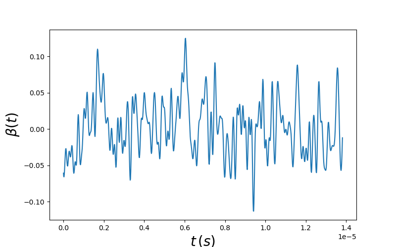
Fig. 7.5.11 A sample charge noise
7.5.2. Dynamics with noise
To simulate the dynamics of our qubit assuming charge noise of the type
described in the previous section, we use the dynamics method
of a QTCAD Noise object
# Simulate dynamic including noise.
num_runs1 = 1 # number of runs to average over
sigz_1run = N.dynamics(H0, delta_V, omega, spectrum, T0, psi0, times,
   qutip.sigmaz(), vec_omega=wk, num_runs=num_runs1)
This method takes several arguments. H0 and delta_V specify the system and
drive Hamiltonians (just as for the noiseless simulations). The charge noise
spectrum is specified using the argument spectrum. T0 is inversely
proportional to the frequency resolution of the discretized noise process
in our simulation (more precisely, T0 sets an artificial period of the
charge noise). psi0 is the initial state of the system, and
times is an array containing the instants in time over which we perform
the simulation. The operator whose expectation value we wish to compute is the
Pauli \(\sigma_z\) operator, i.e. qutip.sigmaz(). The angular frequency
components at which the charge noise spectrum is evaluated is specified as
vec_omega=wk. Finally, the number of simulations (or runs) over which the
expectation value is averaged is specified as num_runs=num_runs1. Above, we
perform a single run, but we may also average over a more statistically
significant number of runs, as shown below.
num_runs2 = 100  # number of runs to average over
sigz_multiruns = N.dynamics(H0, delta_V, omega, spectrum, T0, psi0, times,
   qutip.sigmaz(), vec_omega=wk, num_runs=num_runs2)
We may then plot the results, comparing with noiseless simulations.
# Plot dynamics
fig, axes = plt.subplots(2)
axes[0].plot(result0.times, qutip.expect(qutip.sigmaz(), result0.states),
   label="Without noise")
axes[0].plot(result0.times, sigz_1run, label="With noise")
axes[1].plot(result0.times, qutip.expect(qutip.sigmaz(), result0.states),
   label="Without noise")
axes[1].plot(result0.times, sigz_multiruns, label="With noise")
# Format Plots
axes[0].set_ylabel(f'$\left< \sigma_z (t) \\right>$', fontsize=20)
axes[1].set_ylabel(f'$\left< \sigma_z (t) \\right>$', fontsize=20)
axes[0].set_xlabel(f'$t \, (s)$', fontsize=20)
axes[1].set_xlabel(f'$t \, (s)$', fontsize=20)
axes[0].set_title(f'num_runs = {num_runs1}')
axes[1].set_title(f'num_runs = {num_runs2}')
axes[0].legend(loc='center left', fontsize=16)
axes[1].legend(loc='center left', fontsize=16)
fig.tight_layout()

plt.show()
We obtain the following results.
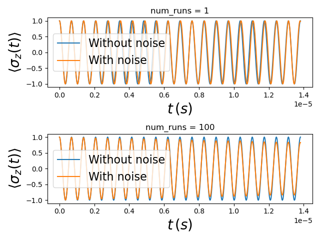
Fig. 7.5.12 Dynamics with and without charge noise
While the single-run simulation results may display variability from simulation to simulation, the average over \(100\) runs exhibits a decay of the Rabi oscillations over time.
7.6. Full code
__copyright__ = "Copyright 2022, Nanoacademic Technologies Inc."

import numpy as np
import pathlib
from matplotlib import pyplot as plt
from device import constants as ct
import qutip
from qubit import spectra, dynamics, noise

# Paths to system and drive Hamiltonians
script_dir = pathlib.Path(__file__).parent.resolve()
path_h0 = str(script_dir/'output'/'h0.npy')
path_u = str(script_dir/'output'/'u.npy')

# Load system and drive Hamiltonians and rewrite in units of hbar = 1
H0 = np.load(path_h0)/ct.hbar
delta_V = np.load(path_u)/ct.hbar

# Define relevant frequencies and time scales of the problem
omega = H0[0,0] - H0[1,1] # qubit frequency
omega_Rabi = np.absolute(delta_V[0,1]) # Rabi frequency on resonance
T_Rabi = 2*np.pi/omega_Rabi # Rabi period

# Define time array
T = 20 * T_Rabi # Total time of the simulations
times = np.linspace(0, T, 1000) # Times at which dynamics are simulated.

# Initialize objects that will handle dynamics and noise.
dyn = dynamics.Dynamics()
N = noise.Noise()

# Simple simulation without noise
# The Hamiltonian H = H0 + delta_V cos(omega*t) in a frame rotating
# at frequency omega.
H = dyn.H_RF(H0, delta_V, omega)

# Solve for the dynamics without any noise.
psi0 = qutip.basis(2, 0) # initial state
result0 = qutip.mesolve(H, psi0, times)

# Plot expectation values of sigma_z and sigma_y as a function of time.
fig, axes = plt.subplots(2)
fig.set_size_inches((8,8))
#<sigma_z (t)>
axes[0].plot(result0.times, qutip.expect(qutip.sigmaz(), result0.states))
#<sigma_y (t)>
axes[1].plot(result0.times, qutip.expect(qutip.sigmay(), result0.states))
# Labels
axes[0].set_ylabel(f'$\left< \sigma_z (t) \\right>$', fontsize=20)
axes[1].set_ylabel(f'$\left< \sigma_y (t) \\right>$', fontsize=20)
axes[0].set_xlabel(f'$t \, (s)$', fontsize=20)
axes[1].set_xlabel(f'$t \, (s)$', fontsize=20)
plt.show()

# Include charge noise which is assumed to affect only the gate which
# generates the drive delta_V.
# Lorentzian spectrum
S0 = 0.01 # Total power
wc = omega_Rabi # Cutoff frequency
w0 = 0 # Central frequency
# T0 should be much larger than the largest time scale of the problem under consideration.
# Used to properly define the Fourier series of the time series related to the noise.
T0 = 50 * T_Rabi  # Must take T0 such that 2*pi/T0 << wc to resolve the spectrum
omega_max = 5*wc
wk = np.arange(0, omega_max , 2*np.pi/T0) + w0
spectrum = spectra.lorentz(wk, S0, wc, w0 = w0)

# Plot spectrum
fig, axes = plt.subplots(1)
fig.set_size_inches((10,6))
axes.plot(wk, spectrum)
axes.set_ylabel(f'$S_\\beta(\omega) \, (s)$', fontsize=20)
axes.set_xlabel('$\omega \, (s^{-1})$', fontsize=20)
axes.set_title('Lorentzian spectral density', fontsize=30)
plt.show()

# Plot time series for the charge noise affecting the gate responsible for
# delta_V.
beta = N.gen_process(times, spectrum, wk, T0)
fig, axes = plt.subplots(1)
fig.set_size_inches((8,5))
axes.plot(times, beta)
axes.set_ylabel(f'$\\beta(t)$', fontsize=20)
axes.set_xlabel('$t \, (s)$', fontsize=20)
plt.show()

# Simulate dynamic including noise.
num_runs1 = 1 # number of runs to average over
sigz_1run = N.dynamics(H0, delta_V, omega, spectrum, T0, psi0, times,
   qutip.sigmaz(), vec_omega=wk, num_runs=num_runs1)

num_runs2 = 100  # number of runs to average over
sigz_multiruns = N.dynamics(H0, delta_V, omega, spectrum, T0, psi0, times,
   qutip.sigmaz(), vec_omega=wk, num_runs=num_runs2)

# Plot dynamics
fig, axes = plt.subplots(2)
axes[0].plot(result0.times, qutip.expect(qutip.sigmaz(), result0.states),
   label="Without noise")
axes[0].plot(result0.times, sigz_1run, label="With noise")
axes[1].plot(result0.times, qutip.expect(qutip.sigmaz(), result0.states),
   label="Without noise")
axes[1].plot(result0.times, sigz_multiruns, label="With noise")
# Format Plots
axes[0].set_ylabel(f'$\left< \sigma_z (t) \\right>$', fontsize=20)
axes[1].set_ylabel(f'$\left< \sigma_z (t) \\right>$', fontsize=20)
axes[0].set_xlabel(f'$t \, (s)$', fontsize=20)
axes[1].set_xlabel(f'$t \, (s)$', fontsize=20)
axes[0].set_title(f'num_runs = {num_runs1}')
axes[1].set_title(f'num_runs = {num_runs2}')
axes[0].legend(loc='center left', fontsize=16)
axes[1].legend(loc='center left', fontsize=16)
fig.tight_layout()

plt.show()