DFT in NanoDCAL

In nanodcal, the Hamiltonian and electronic structure are calculated by a self-consistent field theory. At equilibrium, this SCF theory is precisely DFT. At non-equilibrium, this SCF theory is DFT-like but the density that goes into the SCF is calculated at non-equilibrium by NEGF. Since device modeling involves transport boundary conditions and electrostatic boundary conditions, it is most convenient to use real space DFT. Furthermore, since quantum transport requires various Green’s functions calculated from the device Hamiltonian which involves matrix inversions, it is numerically advantageous to have small Hamiltonian matrices. Due to these considerations, the DFT in nanodcal uses linear combination of atomic orbital (LCAO) basis sets to expand all the physical operators. This Chapter discusses the equilibrium DFT implemented in nanodcal.

The basic theorems of DFT were established by Hohenberg and Kohn [HK64] and Kohn and Sham [KS65], and state that the ground state energy of a system can be uniquely expressed as a functional of the ground state electronic density. In DFT, the electron density is the fundamental quantify from which all quantum mechanical quantities can be calculated. The Kohn-Sham (KS) energy functional is written as:

(13)\[E[\rho]=T[\rho]+\int{d\textbf{r}\rho(\textbf{r}) \left[V_{ext}(\textbf{r})+V_{ion-e}(\textbf{r})\right]+ \frac{1}{2}}\int{d\textbf{r}d\textbf{r}^{\prime} \frac{\rho(\textbf{r})\rho(\textbf{r}^{\prime})}{|\textbf{r}-\textbf{r}^{\prime}|}} +E_{xc}[\rho]\]

where terms correspond to the kinetic energy, the energy of the external potential and the electron-ion potential, the Coulomb interaction between electrons, and the exchange-correlation energy, respectively. If we consider the kinetic energy to be computed in the absence of electron-electron interactions, and apply the variational principle to Eq. (13), we are led to the Kohn-Sham (KS) equation:

(14)\[\left[-\frac{1}{2}\nabla^{2}+\int d\textbf{r}^{\prime} \frac{\rho(\textbf{r}^{\prime})}{|\textbf{r}-\textbf{r}^{\prime}|}+ V_{ion-e}(\textbf{r})+V_{ext}(\textbf{r})+V_{xc}(\textbf{r})\right] \psi_{i}(\textbf{r})=\epsilon_{i}\psi_{i}(\textbf{r})\]

where \(\rho(\textbf{r})\) is the total electron density, \(V_{ion-e}(\textbf{r})\) is the interaction potential between valence electrons and ion cores which are defined by pseudopotential, \(V_{xc}\) is the exchange-correlation functional, and \(V_{ext}\) is any external potential such as the applied external bias potential. The exchange-correlation potential is introduced as:

\[V_{xc}(\textbf{r})=\frac{\delta E_{xc}[\rho]}{\delta\rho(\textbf{r})}\ \ .\]

The terms in brackets of Eq. (14) is identified as the KS Hamiltonian.

The strength of DFT lies in the fact that the interacting many-electron problem has been reduced to a set of KS equations involving non-interacting electrons moving in the effective potential of the other electrons. This mapping is exact provided that the exact exchange-correlation functional is known. Since no one knows the exact form of \(V_{xc}\), approximations must be used in any practical application of DFT. The simplest approximation to the exchange-correlation functional is the local density approximation (LDA) in which one approximates the non-classical corrections to the energy by the energy density of a homogeneous electron gas. The LDA assumes that the exchange-correlation energy at a position \(\textbf{r}\) in an electron gas can be approximated by the exchange-correlation energy in a homogeneous electron gas, \(\epsilon_{xc}^{0}\), having the same density as the electron gas at position \(\textbf{r}\):

\[E_{xc}[\rho(\textbf{r})]=\int\epsilon_{xc}^{0}[\rho(\textbf{r})]\rho(\textbf{r})d\textbf{r}\]

The energy density is typically calculated for high and low density limits and interpolated as a function of the density \(\rho(\textbf{r})\).

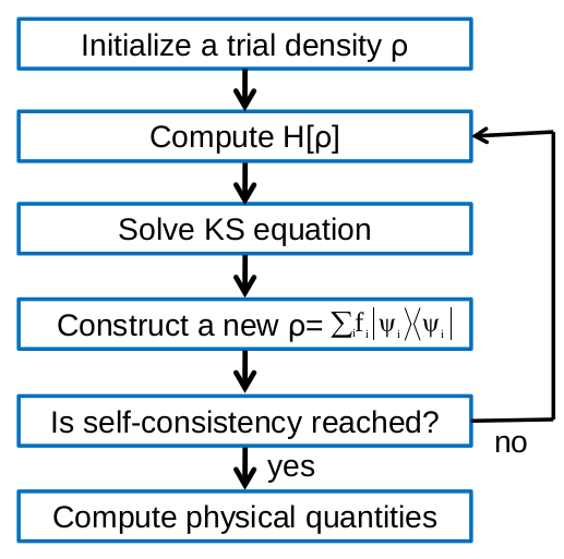
Fig. 13 Flowchart of the self-consistent cycle in a standard DFT calculation.

A flowchart illustrating a self-consistent DFT calculation is shown in Fig. 13. The calculation begins with a trial electron density. The KS Hamiltonian is calculated within a chosen basis set using this initial density. The Hamiltonian is then diagonalized to calculate the eigenvalues and eigenvectors of the system. A new electron density is calculated by populating the eigenvectors according to a Fermi distribution in energy:

(15)\[\rho(\textbf{r})=\sum_{i}f(E_{i},\mu)|\psi_{i}(\textbf{r})|^{2}\]

where \(\mu\) is the chemical potential of the system and chosen such that the total system is charge neutral. Once a new electron density is calculated, the cycle is repeated until self-consistency is achieved. It is useful to emphasize that Fermi-Dirac statistics only apply to systems in equilibrium, and hence the above DFT calculation scheme can not be used for systems under non-equilibrium conditions. Electron transport is amongst the class of non-equilibrium problems, and hence one must go beyond standard DFT when studying transport in order to correctly treat the non-equilibrium quantum statistics of the system. In the next Section, we will discuss how to approach this problem.

LCAO basis functions

In nanodcal, all operators are expanded in terms of LCAO basis functions — called \(\zeta\)-functions. The \(\zeta\) functions are derived from pseudo-eigenstates of the single-atom pseudopotential. By adding a potential barrier, the orbitals become localized in real space. Nanodcal package includes a database of pre-calculated (and tested) \(\zeta\)-functions for most atoms in the periodic table. These were generated by the nanobase atomic package [NAB]. Orbital localization helps to speed up numerical computation but also increases the kinetic energy and changes the eigenvalues slightly. Nevertheless, by choosing the cutoff radius sufficiently large, the localized orbital closely resembles the true pseudo-orbital. After \(\zeta\)-functions are generated, careful tests should be carried out [NAB].

The \(\zeta\)-functions can be classified by the angular momentum \(l\) and associated with angular momentum eigenfunctions \(Y_{lm}\) and an atomic site \(\textbf{R}_{I}\) to form an LCAO basis:

(16)\[\zeta_{\mu}(\textbf{r})=R_{l_{\mu}}(|\textbf{r}-\textbf{R}_{I{}_{\mu}}|) Y_{l_{\mu}m_{\mu}}(\Omega_{\textbf{r}-\textbf{R}_{I{}_{\mu}}})\]

where index \(\mu\) accounts for all quantum numbers \(l_{\mu},m_{\mu}\), and atomic site \(\textbf{R}_{I{}_{\mu}}\). A minimal basis set includes only the \(s,p,d\) orbitals (nine orbital per atom) that may not give enough accuracy for many problems. The default for nanodcal is the double-\(\zeta\) plus polarization (DZP) orbitals [NAB]. Usually, more \(\zeta\) functions provide better accuracy but also requires larger computation. DZP is a reasonable compromise.

Screened form of the KS Hamiltonian

In the KS equation Eq. (14), the potentials may be screened by adding and subtracting the Hartree potential due to a neutral atom charge density \({\displaystyle \int}d\textbf{r}\,\rho^{NA}(\textbf{r}-\textbf{R}_{I})=Z_{I}\) where \(Z_{I}\) is the nuclear charge of atom \(I\). This leaves a screened ion-electron interaction or neutral atom potential, \(V^{NA}\), and a Hartree correction \(V_{\delta H}\) which satisfy:

(17)\[\nabla^{2}V_{\delta H}=4\pi\left[\rho(\textbf{r})-\rho^{NA}(\textbf{r})\right]\]

where

(18)\[\rho^{NA}(\textbf{r})={\displaystyle\sum_{I}}\rho^{{NA,I}} (\textbf{r}-\textbf{R}_{I})\]

and

(19)\[V^{NA}={\displaystyle \sum_{K}}V^{NA,K}(\textbf{r}-\textbf{R}_{K}) ={\displaystyle \sum_{K}}\left\{ V_{{ion-e}}^{K} (\textbf{r}-\textbf{R}_{K})+{\displaystyle \int}d\textbf{r}' \frac{\rho^{NA,K}(\textbf{r}'-\textbf{R}_{K})} {|\textbf{r}-\textbf{r}'|}\right\}\]

where \(K\) labels the atoms. The KS Hamiltonian of Eq. (14) is now of the form:

(20)\[H=\frac{-\nabla^{2}}{2}+\sum_{K}V^{NA,K}(\textbf{r}-\textbf{R}_{K})+V_{\delta H}(\textbf{r})+V_{xc}(\textbf{r})+V_{{ext}}(\textbf{r})\]

There are also long-ranged terms in the total energy: the ion-ion interaction, \(E_{{ ion-ion}}\), and Hartree correction \(\delta E_{H}\). These terms can again be screened by adding and subtracting \(V^{NA}(\textbf{r})\) so that the total energy is now written as [OAS96]:

(21)\[E_{{ tot}}=E_{{ bs}}+\delta E_{\delta{ H}}+\delta U_{{ xc}}+E_{{ sr}}\]

where we have introduced the Hartree correction \(\delta E_{\delta{ H}}\)

(22)\[\delta E_{\delta{ H}}\equiv-{\displaystyle \int}d\textbf{r}\, V_{\delta H}(\textbf{r})\rho^{NA}(\textbf{r})-\frac{1}{2}{\displaystyle \int}d\textbf{r}\, V_{\delta H}(\textbf{r})\left[\rho(\textbf{r})-\rho^{NA}(\textbf{r})\right]\]

the exchange-correlation correction \(\delta U_{xc}\)

(23)\[\delta U{}_{xc}\equiv{\displaystyle \int}d\textbf{r}\,[\epsilon_{xc}(\textbf{r})-V_{xc}(\textbf{r})]\rho(\textbf{r})\]

and the short-ranged (\(sr\)) ionic interaction energy \(E_{{ sr}}\):

(24)\[\begin{split}\begin{array}{rcl} E_{{ sr}} & \equiv & {\displaystyle \sum_{I}}E_{{ sr}}^{I}+\frac{1}{2}{\displaystyle \sum_{I\neq J}}V_{sr}(|\textbf{R}_{I}-\textbf{R}_{J}|)\\ E_{{ sr}}^{I} & = & -\frac{1}{2}{\displaystyle \int\int}d\textbf{r}d\textbf{r}'\,\frac{\rho^{{ NA},I}(\textbf{r})\rho^{{ NA},I}(\textbf{r}')}{|\textbf{r}-\textbf{r}'|}\\ V_{sr}(|\textbf{R}_{I}-\textbf{R}_{J}|) & = & \frac{Z_{I}Z_{J}}{|\textbf{R}_{I}-\textbf{R}_{J}|}-{\displaystyle \int\int}d\textbf{r}d\textbf{r}'\,\frac{\rho^{{ NA},I}(\textbf{r}-\textbf{R}_{I})\rho^{{ NA},J}(\textbf{r}-\textbf{R}_{J})}{|\textbf{r}-\textbf{r}'|},\end{array}\end{split}\]

where indices \(I,J,K\) label the atoms.

Matrix form of the KS equation

By expanding the KS eigenstates \(\psi_{i}\) of Eq. (14) in terms of the atomic orbitals \(\{\zeta_{\nu}\}\) (Eq. (16)):

(25)\[\psi_{i}=\sum_{\nu}c_{\nu}^{i}\zeta_{\nu}(\textbf{r})\]

the KS equation Eq. (14) is transformed to an equivalent tight-binding matrix problem:

(26)\[H_{\mu\nu}c_{\nu}^{i}=\epsilon_{i}S_{\mu\nu}c_{\nu}^{i}\]

where \(S_{\mu\nu}\) is the overlap matrix elements. Analogously, In Chapter 3 the Green’s function \(G\) satisfies a matrix equation:

(27)\[G_{\nu^{\prime}\nu}(E)=\delta_{\mu\nu}\]

where \(E\) is the electron energy. More on Green’s function formulation can be found in Chapter 3.

The Hamiltonian and overlap matrix elements are defined by the following:

(28)\[\begin{split}\begin{array}{rcl} H_{\mu\nu} & \equiv & {\displaystyle \int}d\textbf{r}d\textbf{r}'\,\zeta_{\mu}^{*}(\textbf{r}){\huge[}\\ \hspace{1.0cm} & & \delta(\textbf{r}-\textbf{r}')\times\left[-\frac{\nabla_{\textbf{r}'}^{2}}{2}+\sum_{K}V^{{ NA},K}(\textbf{r}-\textbf{R}_{K})+V^{eff}(\textbf{r})\right]\\ & & \hspace{1.0cm}+\sum_{K}V_{K}^{nl}(\textbf{r}-\textbf{R}_{K},\textbf{r}'-\textbf{R}_{K}){\huge]}\zeta_{\nu}(\textbf{r}')\\ S_{\mu\nu} & \equiv & {\displaystyle \int}d\textbf{r}\,\zeta_{\mu}^{*}(\textbf{r})\zeta_{\nu}(\textbf{r})\ .\end{array}\end{split}\]

In the above, we have defined an effective potential \(V^{eff}\):

(29)\[V^{eff}(\textbf{r})\equiv V_{\delta{ H}}(\textbf{r})+V_{xc}(\textbf{r})\]

We have also explicitly written out the non-local (\(nl\)) part of the pseudopotential \(V_{K}^{nl}(\textbf{r}-\textbf{R}_{K},\textbf{r}'-\textbf{R}_{K})\).

The size of these matrices can be determined. For a system with \(N_{A}\) atoms and assuming each atom has the same number \(N_{\zeta}\) basis functions, then the matrix size is \((N_{A}N_{\zeta})\times(N_{A}N_{\zeta})\). Of course, when \(N_{\zeta}\) is different from atom to atom, one has to add up to obtain the total number of orbitals in order to calculate the matrix size. Hence, for 500 atoms each having 20 \(\zeta\)-functions, the matrix size is \(10,000\times10,000\). Such matrices can be diagonalized without too much difficulty. For isolated or periodic systems, nanodcal solves the KS equation Eq. (26) by matrix diagonalization.

Matrix elements

The individual terms of the Hamiltonian matrix Eq. (28) are listed below and evaluated numerically:

(30)\[\begin{split}\text{Overlap: } & S_{\mu\nu} & \equiv & {\displaystyle \int}d\textbf{r}\,\zeta_{\mu}^{*}(\textbf{r})\zeta_{\nu}(\textbf{r})\\ \text{Kinetic energy: } & T_{\mu\nu} & \equiv & {\displaystyle \int}d\textbf{r}\,\zeta_{\mu}^{*}(\textbf{r})\frac{-\nabla^{2}}{2}\zeta_{\nu}(\textbf{r})\\ \text{Neutral atom potential: } & V_{\mu\nu}^{NA} & \equiv & {\displaystyle \sum_{K}\int}d\textbf{r}\,\zeta_{\mu}^{*}(\textbf{r}) \times V^{{ NA},K}(\textbf{r}-\textbf{R}_{K})\zeta_{\nu}(\textbf{r})\\ \text{Non-local pseudopotential: } & V_{\mu\nu}^{nl} & \equiv & {\displaystyle \sum_{K}\int}d\textbf{r}\, d\textbf{r}'\zeta_{\mu}^{*}(\textbf{r}) \times V_{K}^{nl}(\textbf{r}-\textbf{R}_{K},\textbf{r}'-\textbf{R}_{K})\zeta_{\nu}(\textbf{r}')\\ \text{Effective potential: } & V_{\mu\nu}^{eff} & \equiv & {\displaystyle \int}d\textbf{r}\,\zeta_{\mu}^{*}(\textbf{r})V^{eff}(\textbf{r})\zeta_{\nu}(\textbf{r})\end{split}\]

The first four expressions only need to be computed once and nanodcal calls them “rigid atomic potential” because they do not change during the DFT self-consistent iteration. On the other hand, \(V_{\mu\nu}^{eff}\) must be evaluated in each self-consistent step because this potential is a functional of the self-consistent charge density \(\rho(\textbf{r})\) through Eq. (29).

k-sampling

Nanodcal does k-sampling for periodic systems which is made of periodic units of identical super-cells. A super-cell can be the smallest primitive cell or any cell that can be periodically extended to form the bulk crystal. With k-sampling, the KS eigenstates \(\psi_{i}\) or its expansion coefficients \(c_{\nu}^{i}\) in Eq. (25), and the KS eigenvalues \(\epsilon_{i}\) of Eq. (26), all pick up another index \(k\) whose value is sampled within the first Brillouin zone. Similarly, the Green’s function in Eq. (27) also picks up the k index.

Solution of the KS equation

The solution process of the self-consistent Kohn-Sham equation is plotted in Fig. 13. The self-consistent iteration starts with an initial guess for the density matrix and, from it, the initial KS Hamiltonian is constructed by evaluating Eq. (29) and the matrix elements Eq. (30). From the KS Hamiltonian matrix, nanodcal solves Eq. (26) by direct matrix diagonalization to obtain the KS eigenfunction coefficients \(c_{\nu}^{i}\), and then an output density matrix is formed from these coefficients. If the output density and input density matrices do not match, a new input density is formed based on the output density matrix, using Eqs. (25) and Eq. (15). This process is repeated until self-consistency is achieved. Data analysis is then performed and physical quantities calculated from the electronic ground state. Afterward, the external variables such as the nuclear positions \(\{\textbf{R}_{I}\}\) are updated and a new self-consistent calculation is performed. Each step of Fig. 13 is briefly discussed below.

The default initial density in nanodcal is a superposition of neutral atom densities:

\[\rho^{NA}(\textbf{r})=\sum_{I}\rho^{{ NA,I}}(\textbf{r}-\textbf{R}_{I})\]

On the other hand, the self-consistent density based on a previous calculation can be read into nanodcal to start a new calculation. Similarly, users can prepare other initial densities to be read into nanodcal to start a calculation.

In nanodcal, the calculation of \(V^{eff}(\textbf{r})\) requires a real space grid. From a given charge density \(\rho(\textbf{r})\), the self-consistent part of \(H[\rho]\), i.e. \(V^{eff}(\textbf{r})\) of Eq. (29), is obtained by solving the Poisson equation Eq. (17) for the Hartree potential and adding to it the exchange-correction potential \(V_{xc}\). The Poisson equation is solved by 3D FFT, 2D FFT plus real space method in the third dimension, or 3D real space multi-grid method, depending on problems. For \(V_{xc}\), nanodcal uses LDA, LSDA and various GGA functionals. From the obtained \(V^{eff}(\textbf{r})\), the matrix elements Eq. (28) must be calculated.

The output density matrix \(\hat{\rho}\) is a functional of the input Hamiltonian matrix \(\hat{H}\) and overlap matrix \(\hat{S}\). The exact relationship between them will depend on the boundary conditions on the system. For usual equilibrium DFT total energy calculations the density matrix \(\rho\) is given by the KS eigenstates \(\psi_{i}\):

\[\rho(\mu,\beta)\equiv e^{-\beta(H-\mu)}={\displaystyle \sum_{i}}\left|\psi_{i}\rangle f^{{ EQ}}(E-\mu;\beta)\langle\psi_{i}\right|\]

where \(\beta\) is the electron temperature, \(\mu\) the chemical potential, and

\[f^{{ EQ}}(E-\mu;\beta)=\frac{1}{1+\exp(\beta(E-\mu))}\]

is the familiar Fermi function. The chemical potential is defined by the charge neutrality condition:

\[Tr[{\rho}(\mu,\beta)]=N\]

In terms of the KS wavefunctions \(\{\psi_{i}\}\), the expectation value of any operator \({A}\) is given by:

\[\langle{A}\rangle={\displaystyle \sum_{i=1}^{N}}\langle\psi_{i}|{A}|\psi^{i}\rangle.\]

In terms of the density matrix, the same expectation value is given by

\[\langle{A}\rangle=Tr[{\rho}{A}]\]

For example, the KS band-structure energy and total charge are given by:

\[\begin{split}\begin{array}{rcl} E_{{ BS}} & = & Tr[\hat{\rho}\hat{H}]\\ N & = & Tr[\hat{\rho}\hat{S}]\end{array}\end{split}\]

The real space density is the diagonal part of the density matrix in the position representation, \(\rho(\textbf{r},\textbf{r})\).

During the self-consistent solution process of the KS equation, i.e. the loop in Fig. 13, in principle the output density matrix of the previous step can be used as the input to the next self-consistent step. But such a procedure causes large charge fluctuations that make convergence difficult. Therefore one needs to mix the new density with the old density in some way. One can also mix the new potential with the old potential. For example, in a simple linear mixing,

(31)\[\rho^{(n+1)}\rightarrow(1-\alpha)\rho^{(n)}+\alpha\rho^{(n+1)}\]

where \(0<\alpha<1\). The simple mixing is slow because \(\alpha\) is usually very small. One can use several more sophisticated mixers such as the Broyden method, Pulay method, etc.. One can choose these methods in nanodcal.

Summary

This chapter reviews the equilibrium DFT equations implemented in nanodcal for typical total energy electronic structure calculations. Using the LCAO basis, the KS equation is solved by direction matrix diagonalization. The method in this chapter is used for solving finite systems such as a molecule, or periodic systems such as a crystalline solid. In the next chapter, we shall review the non-equilibrium calculations of nanodcal that is used non-equilibrium quantum transport modeling.

[HK64]

Hohenberg, P., & Kohn, W. (1964). Inhomogeneous electron gas. Physical Review, 136(3B), B864.

[KS65]

Kohn, W., & Sham, L. J. (1965). Self-Consistent Equations Including Exchange and Correlation Effects. Physical Review, 140(4A), A1133.

[OAS96]

Ordejón, P., Artacho, E., & Soler, J. M. (1996). Self-consistent order density-functional calculations for very large systems. Physical Review B - Condensed Matter and Materials Physics, 53(16), R10441–R10444.

[NAB] (1,2,3)

Nanobase is an atomic package of Nanoacademic Technology Inc.. See, Nanobase User Reference at www.nanoacademic.com.