7. Diamond vacancy defect tutorial
7.1. Introduction
In this tutorial, I explain how to calculate the defect level diagram of a carbon vacancy in diamond. We will calculate the formation energy as a function of chemical potential of several charge states of the defect. The formation energy of a charged defect is given by
\(E_f[D^q] = E[D^q] - E[Host] - \sum n_s \mu_s + q E^{Fermi} + E_{corr}(q,\epsilon)\)
where \(E[D^q]\) is the total energy of the defect system with charge q, \(E[Host]\) is the total energy of the perfect system, \(n_s\) is the number of atoms of species \(s\) added (if positive) or removed (if negative). For instance, in the diamond vacancy, we have \(n_C = -1\). \(\mu_s\) is the chemical potential of species \(s\), \(E^{Fermi}\) is the chemical potential of the electrons and \(E_{corr}(q,\epsilon)\) is a correction that account for finite size effects. I will use the correction scheme of Kumagai and Oba, which requires determining the dielectric constant of diamond (and more generally the dielectric tensor).
After obtaining the defect formation energies of several charge states, we will compute the following transition level diagram
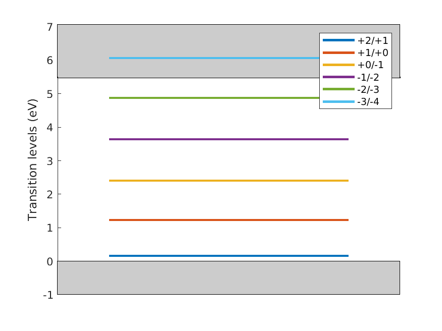
Fig. 7.1.1 Carbon vacancy level diagram
I shall go through the following steps:
In this tutorial, I will use 64-atom supercells and neglect structure relaxation to minimize the computational intensity.
7.2. Vacuum atom
Since we will investigate a vacancy defect with atomic orbitals, we will
introduce a so-called vacuum atom in place of the removed carbon atom.
Simply put, we remove the pseudopotential but keep the orbitals. I
create a vacuum atom from the pseudopotential file C_SZDP.mat as
follows
load('C_SZDP.mat')
data = makeVacuum(data);
save Va_SZDP data
In what follows, a carbon vacancy will draw its atomic orbital basis
from the file Va_SZDP.mat, and I shall use Va to label the
element.
7.3. Neutral defect band structure
In this section, I compute the band structure of the neutral vacancy in diamond. This is to give myself an idea of the electronic structure of the defect, which will determine how we do things next. As we shall see, the diamond vacancy has a six-fold degenerate defect state (including spin degeneracy). But the finite supercell size yields an artificial dispersion of the defect levels across the Brillouin zone. This so-called band dispersion error is mitigated using a uniform occupation scheme instead of, say, Fermi-Dirac occupancies.
So we need to know the band structure to know how to populate it. We
thus perform the ground state calculation scf.input and get a band
structure from bs.input. The band structure looks like
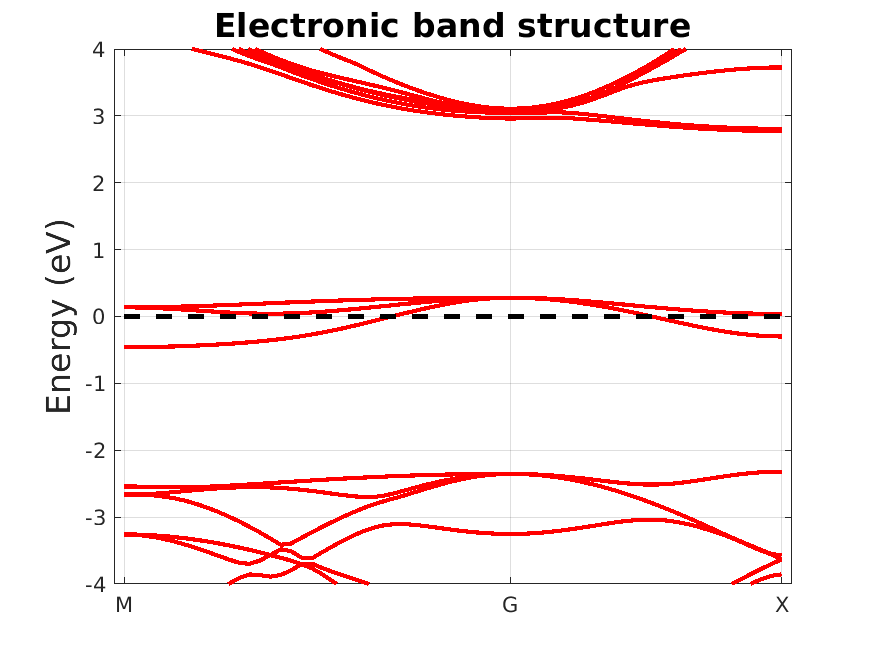
Fig. 7.3.1 Neutral defect band structure
The Fermi level clearly cuts through three defect bands around the center of the band gap. In the limit of an infinite system size, the three bands become flat and degenerate (as they are at the \(\Gamma\)-point). The dispersion is a finite size effect. Further inspecting the eigenvalues and occupancies reveals that the neutral defect level is 1/3 occupied. To mitigate the (incorrect) dispersion effects, we will adopt is fixed population scheme to force the occupancy to 1/3 across the entire Brillouin zone, as it would in the infinite size system. This not only improve convergence with respect to supercell size, but also with respect to k-sampling, as shown in this figure
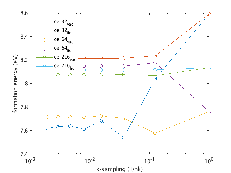
Fig. 7.3.2 Neutral defect k-sampling convergence
Here, the subscript vac is for the regular occupancy scheme and fix for the fixed occupancy scheme.
7.4. Neutral formation energy
Now that I know the electronic structure, I’m ready to perform the
supercell calculations. First, we’ll need the pristine system potential
for reference. I thus set up a bulk supercell as bulk/scf.input.
Note the following parameter is set as follows
option.savePotential = 1
to make sure to save the potential.
Next, let’s see what’s in the neutral directory. The script scf.input defines
the parameters for the ground state calculation of the neutral defect.
The important keywords are at the bottom of the file
nv = 64 * 4 - 4
atom.nvalence = nv - 0
kpoint.sampling = 'fixed'
kpoint.nocc = [ones(floor(nv/2)-1,1);2/6;2/6;2/6]
element(2).species = 'Va'
element(2).path = '../Va_SZDP.mat'
First nv is not a keyword, but simply a useful variable to write the
rest of the file. It corresponds to the total valence of the neutral
defect system, i.e. 64 atoms times 4 electrons, minus 1 atom times 4
electrons. The keyword atom.nvalence is set to nv - 0. We could
simply set it to nv but this is to make it obvious that the system
is neutral; later we’ll change 0 for something else when we study
charged defects. The fixed occupancy is defined using the keywords
kpoint.sampling and kpoint.nocc. The value of
kpoint.sampling is self-explanatory. For kpoint.nocc, one needs
to specify the occupancy of each band. In a vacancy defect system, there
are floor(nv/2)-1 fully occupied bands, three partially occupied
bands and then unoccupied bands. We only need to specify the occupancy
of the (partially) occupied bands. I thus use the MATLAB function
ones to generate a floor(nv/2)-1-entry vector of ones (the spin
factor should not be included here). The following three defect levels
should then be populated with 1/3 electron each, for a total of nv/2
electrons (again neglecting the spin factor). Finally, we add the vacuum
atom definition with label Va. Note that this is all done in a
programmatic way, but you could input all numbers in a more manual way
if that makes you feel more comfortable.
Once the scf.input calculation is done, we can proceed to compute
the formation energy of the neutral defect. This is done by the
baseFormEnergy function. We must create a structure to store the
following parameters:
The chemical potential (see the Chemical potential tutorial).
The species occupancy, i.e. how many atoms of each species are added or removed.
The fermi level, which we pick as the VBM here (see Valence band maximum tutorial).
This is done as follows
param.n = [-1];
param.mu = [-163.887300];
param.efermi = 10.126067;
ef = bareFormEnergy('bulk/results/scf','neutral/results/scf',param);
fprintf('ef = %f eV\n',ef);
which prints
ef = 7.808313 eV
Note the data in param are in units of eV. Usually, one includes
ionic relaxation in the formation energy contribution by using the total
energy of the relaxed defect supercell. If you have the time and
resources, you may do the computation rlx.input instead of
scf.input.
7.5. Charged defect formation energy
We now proceed to a charged defect formation energy. Charged defect
supercell calculations are quite similar to the neutral defect one. The
main difference is that we will use a correction formula to mitigate
finite-size electrostatic errors. Let’s take the +2 charged defect for
example (i.e. change directory to plus2). There is an input file
scf.input quite similar to that of the neutral defect. It ends as
follows
nv = 64 * 4 - 4
atom.nvalence = nv - 2
kpoint.sampling = 'fixed'
kpoint.nocc = [ones(floor(nv/2)-1,1);0/6;0/6;0/6]
element(2).species = 'Va'
element(2).path = '../Va_SZDP.mat'
As before nv is not a keyword but a variable which corresponds to
the total valence of the neutral defect system. The keyword
atom.nvalence is set to nv - 2; we remove two electrons making
the total charge +2. The occupancy is defined using the keywords
kpoint.sampling and kpoint.nocc. Remember that the three defect
levels of the neutral defect were populated with 1/3 electron each. Here
we remove two electrons (one in each spin channel) from those levels
leaving zero electron. We thus set the occupancy of the last three bands
to 0/6 (to keep the template file intact). Finally, we add the
vacuum atom definition with label Va.
As before, the (bare) formation energy may be obtained with
bareFormEnergy
param.n = [-1];
param.mu = [-163.887300];
param.efermi = 10.126067;
ef = bareFormEnergy('bulk/results/scf','neutral/results/scf',param);
fprintf('ef = %f eV\n',ef);
which yields
ef = 6.875340 eV
Now, this formation energy includes defect-defect electrostatic
interactions which shouldn’t be present in the infinite-size, isolated
defect system. Here, I’ll use the the correction scheme of Kumagai and
Oba, which requires determining the dielectric constant of diamond. This
may be done following the Dielectric constant tutorial. In the end, one gets a
value close to 5.41. The electrostatic correction is performed by
the function corrKO as follows
param.dielectric = 5.41*[1,0,0;0,1,0;0,0,1];
param.site = 1;
ec = corrKO('bulk/results/scf','plus2/results/scf',param);
fprintf('ec = %f eV\n',ec);
which yields
ec = 0.765893 eV
It is quite significant indeed, more than 10%. The interface of
corrKO is similar to that of bareFormEnergy, but it requires
different parameters. First, the dielectric tensor is required in
param.dielectric. Here it is set to 5.41 times the identity matrix.
Next, param.site is the atom index corresponding to the center of
the defect (here the vacancy). The total formation energy is finally
ef + ec = 7.641232 eV.
Again, one should usually include ionic relaxation in the formation energy contribution by using the total energy of the relaxed defect supercell.
7.6. Transition level diagram
In this section, we derive the transition level diagram from the defect formation energy. Out starting point is the corrected formation energy for all charged states. If you repeat the steps from the previous section for all charged states, you should find values close to
ef = [5.746588,6.592742,7.808313,9.448148,11.544052,14.094930,17.067092];
for the bare formation energy and
ec = [0.681561,-0.010808,0.000000,0.760446,2.300168,4.624176,7.712705];
for the corrections, which gives finally
ef = [6.428149,6.581935,7.808313,10.208593,13.844220,18.719106,24.779797];
You can read everything using the script readall.m. Recall the
formula for the formation energy of a defect is
\(E_f[D^q] = E[D^q] - E[Host] - \sum n_s \mu_s + q E^{Fermi} + E_{corr}(q,\epsilon)\)
Therefore, as we vary \(E^{Fermi}\) the most energetically favorable
charge state will change. The crossing point between the formation
energy of a charged state and another is a transition level. Those
levels can be computed by the function transitionLevels.
ef = [6.428149,6.581935,7.808313,10.208593,13.844220,18.719106,24.779797];
q = [2,1,0,-1,-2,-3,-4];
trlvl = transitionLevels(q,ef);
Note that if the data is not in decreasing q-order,
transitionLevels will reorder the data internally. The first entry
in trlvl is thus the transition level between the highest charge
state and the second highest, and so on.
I get
trlvl = [0.153786,1.226378,2.400280,3.635627,4.874886,6.060691];
in units of eV for the transition levels. This means that the first
transition (+2/+1) occurs below the VBM and the last transition (-3/-4)
above the CBM. Finally, this is vizualize calling the function
plotTLD. One just needs to set the band gap (experimental or else)
in param.gap as follows
param.gap = 5.47
plotTLD(q,trlvl,param)
which produces the following plot
Fig. 7.6.1 Transition level diagram of diamond