6. Dielectric constant tutorial
6.1. Introduction
In this tutorial, you will see how to compute the dielectric constant of diamond using an external electric field. In essence, the electrons react to the introduction of an external field by screening it. By looking at the variation of the effective (Kohn-Sham) potential we can determine by how much. The ratio of the external potential to the effective potential variation is the dielectric constant.
6.2. The calculations
We introduce a sawtooth potential, which has the virtue of being periodic and linear away from the bends, making the analysis straightforward.
We first perform the calculation defined in scf_bulk.input, which
will yield the reference effective potential. Note the lines
option.replicateCell = [1,1,8]
option.savePotential = 1
The input file scf_bulk.input defines a conventional cubic unit cell
of diamond. But the keyword option.replicateCell tells RESCU to set
up a \(1 \times 1 \times 8\) supercell calculation. Then
option.savePotential is set to 1 so that the potential terms are
saved before exiting the program.
We then perform the calculation defined in scf_vext.input, which
will yield the screened effective potential. Note the lines
potential.external = @(u,v,w) sawtooth(0.5,u,v,w,3)
rho.in = 'results/scf_bulk'
The keyword potential.external allows introducing an external
potential as a function handle. Here sawtooth is a user defined function
whose arguments are: amplitude, u-grid, v-grid, w-grid and dimension. It
should be found in src. The amplitude is in units of eV. The u-grid,
v-grid, w-grid are fractional coordinate grids. The dimension is 3,
meaning that the sawtooth function runs along the third lattice vector
direction. Finally, we set rho.in to results/scf_bulk to restart
from the bulk results.
6.3. Determine the dielectric constant
The last step is to extract the dielectric constant from the potentials.
This is done with the script read_eps.m. Basically, the script does
the following
Load the potentials.
Perform a linear fit of the external potential in the center of the linear potential region.
Perform a linear fit of the effective potential in the center of the linear potential region.
Determine the dielectric constant as the ratio of the two.
Finally, it will print
dielectric constant = 5.410509
You may also plot the potentials and fit as follows
figure(); hold on
z = w * avec(3,3);
tmp = squeeze(mean(mean(reshape(vext, fgn),1),2));
plot(z,tmp, '--', 'DisplayName', 'v_{ext}'); hold on
tmp = squeeze(mean(mean(reshape(vel - velb, fgn),1),2));
plot(z,tmp, '--', 'DisplayName', '\Delta V'); hold on
vext = sawtooth(0.5/p1(1)*p2(1),u3,v3,w3,3);
tmp = squeeze(mean(mean(reshape(vext, fgn),1),2));
plot(z,tmp, '--', 'DisplayName', 'v_{fit}'); hold on
xlabel('z (bohr)')
ylabel('potential (Ha)')
legend(); grid on
saveas(gcf,'vext_diamond.png')
which gives
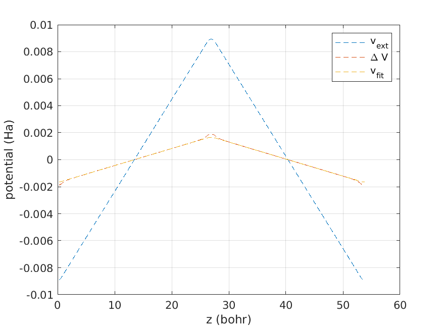
Fig. 6.3.1 Potential screening in diamond