Crystals

A crystal is a bulk structure consisting of repeated units periodically extended in one to three dimensions. An infinitely long wire is an 1d crystal; an infinitely large film is a 2d crystal; and an infinitely large 3d structure is a 3d crystal. Many DFT packages are for calculating these periodic systems. The Bloch theorem allows one to focus on a single repeating unit of an infinitely large periodic crystal by the k-sampling technique.

The smallest unit in a periodic crystal is a primitive cell. For instance the primitive cell of Si has two Si atoms; the primitive cell of Fe has one atom, etc. Once the atomic positions of the atoms inside the primitive cell is specified, lattice vectors are used to periodically extend the primitive cell to infinity forming a crystal. Therefore one has to define these lattice vectors. Since the primitive cell is the smallest unit, it is desirable to use primitive cell in DFT calculations to save some computation time. It is true that the smaller the cell is, the larger the number of k-sampling is needed. But even using large enough k-sampling will still save some time. On the other hand, since we are dealing with a periodic crystal, we can actually use any unit-cell (called supercell) as our basic unit to extend to the full infinitely large crystal. These supercells typically have more atoms than that contained in the primitive cell, thus the computation will cost more time. For cubic crystals, it is some times simpler to set up atomic positions of a supercell having a cubic shape.

Similar to that discussed in section Molecules, NanoDCAL solves the Kohn-Sham equation for the supercell inside a computation box of linear dimensions \((L_x,L_y,L_z)\). Because we are dealing with a periodic structure, the values of \((L_x,L_y,L_z)\) must guarantee periodicity when extended to form the crystal. Fig. 5 is a 2d schematic of a bulk crystal.

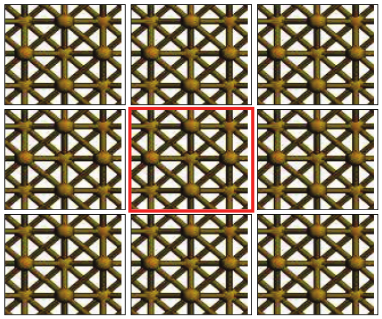
Fig. 5 Schematic diagram of a supercell (the cell in the centre) containing a crystal struc- ture. The supercell is periodically extended in 1, 2 or 3 dimensions to form an 1d, 2d, or 3d crystal.

Basic input file

The basic input file for bulk calculation is very similar to that of molecule calculation discussed section Molecules. There are some special points to be noted and we will focus on them in the following discussions. There are several examples of bulk calculations and let’s go to /examples/Group2_Fe_Bulk/ which is for computing electronic structure of Fe crystal. Fe scf input shows the scf.input for the bulk Fe calculation.

Since Fe is a magnetic metal, line-3 of Fe scf input indicates that this is a collinear spin calculation. Line-4 uses Matlab function eye(3) to set up a \(3\times 3\) identity matrix, and then multiply it by 5.22 au. This is to set up the supercell vectors to be 5.22 au in all three dimensions. Here, the atomBlock has two Fe atoms forming the supercell. For BCC structure, one Fe atom sits at the origin and the other at the body centred location. A new parameter appears in line-6, i.e. the keyWord SpinPolarization. Spin polarization is defined as,

\[\eta \ \equiv \frac{Q_\uparrow - Q_\downarrow}{Q_\uparrow + Q_\downarrow} :label: spin-polar\]

where \(Q_{\uparrow,\downarrow}\) are charges in the spin-up and -down channels. For spin dependent calculations, it is usually helpful to give some initial value to \(\eta\) and here \(\eta = 0.2\). During the DFT iterations, \(\eta\) will be determined self-consistently. Lines 10-11 indicate the units to be used, thus the numbers in the atomBlock are in au. Please refer to Section Default units for the default units. Here we override the default by lines 10-11.

Finally, lines 12-14 tells nanodcal to do self-consistent DFT iterations using the multisecant mixing method [ML08]. Refer to Input reference section for more details.

1. The input file scf.input for bulk Fe calculation:

Listing 3 Fe scf input

% The input file for the self-consistent field (hamiltonian) calculation.
% The file Fe_DZP.nad is needed for the calculation.
% type "nanodcal -parameter ? \.SCF\." for a complete list of input parameters
% which are used for the SCF calculation.
% no default value for the calculation name; must be given.
calculation.name = scf
% type "nanodcal -parameter ? calculation.name" for a complete list of
% calculation names.
% some parameters to define the system
system.name = ’FeBulk’
system.spinType = ’CollinearSpin’
system.centralCellVectors = eye(3)*5.2202
system.atomBlock = 2
AtomType X
Y
Z orbitaltype SpinPolarization
Fe 0.000000 0.000000 0.000000 DZP
0.200000
Fe 2.610100 2.610100 2.610100 DZP
0.200000
end
% type "nanodcal -parameter ? system\." for a complete list of input
% parameters which are used to define the system.
% the length and evergy units used for the input and output.
calculation.control.lengthUnit = ’au’
calculation.control.energyUnit = ’au’
% some parameters for SCF calculation
calculation.SCF.mixer.class = cMixerMultiSecant
calculation.SCF.mixer.parameter.beta = 2e-1
calculation.SCF.mixer.parameter.maxhistory = 3
% type "nanodcal -parameter ? \.SCF\." for a complete list of input parameters
% which are used for the SCF calculation.

2. Standard output of the Fe bulk run:

Listing 4 Fe scf output

System Summary:
System Name: FeBulk
System Type: periodic-3D, collinear spin
System Symmetry: Oh
# of Atoms in Central Cell: 2
# of Electrons of Central Cell Atoms: 16
# of Basis of Central Cell Atoms: 30
Parameters Summary:
XC functional type: LDA_PZ81
central cell base vectors:
v1 = (5.220200e+000, 0.000000e+000, 0.000000e+000)
v2 = (0.000000e+000, 5.220200e+000, 0.000000e+000)
v3 = (0.000000e+000, 0.000000e+000, 5.220200e+000)
realspace grid numbers: [17 17 17]
realspace grid volume: 0.028954 Bohr3̂
k-space grid numbers: [15 15 15]
electronic temperature: 100 K
....

Basic standard output

As already demonstrated in Section Basic standard output, we run the Fe bulk calculation by typing:

nanodcal scf.input

Many lines of output appear on the computer screen similar to those shown in Benzene output. Fe scf input (b) shows the system and parameter summary blocks of the standard output. In particular, since we have given a name to this run in scf.input, line-2 of Fe scf output (b) presents it. Line-3 indicates that it was a periodic 3d bulk run with collinear spin configuration. Lines 4-6 are similar to that in Benzene output.

In the parameter block, only line-14 is new in comparison to Listing 2. Since Listing 2 is for a molecular calculation, there is no k-sampling. But for the bulk Fe run, it is a periodic system and appropriate k-sampling must be done. Thus, line-14 of Fe scf output indicates that we did k-sampling using a k-grid of \([15,15,15]\) points. How did NanoDCAL decide the k-grids? Again, as discussed in Section Basic standard output, NanoDCAL sets up k-grid by a precision control parameter:

calculation.control.precision = low, or normal, or high

These precision parameters tell NanoDCAL the numerical accuracy to be enforced. In Section Basic standard output we discussed how this affects the energy cutoff that determines the real space grid (see (1) and associated discussions), here we see how the k-grid is determined. In particular, if scf.input does not specify what precision to use, nanodcal applies the default which is ‘normal’. For k-grids, low, normal or high precisions mean 20 Bohr, 40 Bohr and 80 Bohr upper cutoff for 1/k values. As a result, it was decides that k-grid should be \(15^3\) points for normal precision as shown in Fe scf output. On the other hand, the user can enforce his own k-grid by adding the following keyWord in scf.input:

calculation.k_spacegrids.L_cutoff = 55

this lines enforces a higher cutoff of 55 Bohr than the default normal precision of 40 Bohr. As a result, the k-grid will become \(21^3\) instead of \(15^3\) for the Fe example. One can also directly tell NanoDCAL what k-grid to use by adding the following line to scf.input:

calculation.k_spacegrids.number = [8 12 14]

This would set up a k-grid of 8 points in \(k_x\), 12 points in \(k_y\) and 14 in \(k_z\).

Finally, the actual self-consistent iteration proceeds just like that in Listing 2 discussed in Section Basic standard output, and will not be repeated here. In addition, for bulk systems the essential output files of nanodcal are the same as that shown in Table 5.

Calculating band structure

Once the SCF computation is converged, one may wish to obtain the band structure of the crystal. In the /examples/Group2_Fe_Bulk/ directory, you can find a four line input file band.input for this purpose, as shown below:

% The input file for the electronic structure (band structure) calculation.
% The crystal structure is automatically determined by the code.
% The file NanodcalObject.mat is needed for the calculation.
% type "nanodcal -parameter ? calculation.bandstructure" for a complete list
% of input parameters which are used for the band structure calculation.
% the hamiltonian of the cNA_LCAO object saved in the file
% NanodcalObject.mat will be used for the calculation.
system.object = NanodcalObject.mat
% Another way to define the hamiltonian is through the input parameter
% system.hamiltonian.
% type "nanodcal -parameter ? system\." for a complete list of input
% parameters which are used to define the system.
% no default value for the calculation name; must be given.
calculation.name = bandstructure
% type "nanodcal -parameter ? calculation.name" for a complete list of
% calculation names.
% some input parameters for the calculation.
calculation.control.energyUnit = eV
calculation.bandStructure.plot = 1
% type "nanodcal -parameter ? calculation.bandstructure" for a complete list
% of input parameters which are used for the band structure calculation.

Here, line-1 tells NanoDCAL to start from an object file obtained from a previous self-consistent DFT run. Line-2 requires a calculation of band structure. Line-3 requires the energy unit to be eV in the present calculation. Note that even though we used atomic unit for the SCF run (see Fe scf input), line-3 here will convert it to eV during the present band structure calculation and, hence, line-4 shall plot a figure using eV as energy unit. Type:

nanodcal band.input

a band structure of the Fe crystal is produced and plotted. The band structure calculation uses the same control parameters stored in the system object output file NanodcalObject.mat. Note that NanoDCAL does band unfolding automatically so that the plotted bands are already unfolded.

Now, we return to entry 5 of Table 5, namely the output file CalculatedResults.mat. Because we have calculated band structure of Fe, this file now contains the information about the band structure. By loading this file into Matlab, you can examine the stored data by typing the following in the Matlab command window:

load CalculatedResults.mat
data
data.bandStructure
data.bandStructure.data
...

Here, each line provides increasingly more information.

Calculating complex band structure

In typical electronic calculations, one is after the band structure of the crystal. For quantum transport, one may be interested in the complex band structure. A complex band structure is \(E=E(k_1,k_2,k_3)\) where any of the \(k_i\) is a complex value. Why complex band structure is interesting? For example, suppose an electron tunnels into the band gap of an insulator: its wave function becomes evanescent and it’s \(k\) becomes an imaginary hence complex number. Complex bands can connect real bands across the band gap.

In the /examples/Group2_Fe_Bulk/ directory, there is an input file cband.input which essentially has the following lines:

% The input file for the complex-band structure calculation.
% The file NanodcalObject.mat is needed for the calculation.
% type "nanodcal -parameter ? complexBandStructure" for a complete list
% of input parameters which are used for the complex-band structure
% calculation.
% the hamiltonian of the cNA_LCAO object saved in the file
% NanodcalObject.mat will be used for the calculation.
system.object = NanodcalObject.mat
% Another way to define the hamiltonian is through the input parameter
% system.hamiltonian.
% type "nanodcal -parameter ? system\." for a complete list of input
% parameters which are used to define the system.
% no default value for the calculation name; must be given.
calculation.name = cbs
% type "nanodcal -parameter ? calculation.name" for a complete list of
% calculation names.
% some input parameters for the calculation.
calculation.control.energyUnit = eV
calculation.complexBandStructure.plot = true
calculation.complexBandStructure.energyPoints = -20:0.1:20
calculation.complexBandStructure.numberOfKpoints = [1 1 1]
% type "nanodcal -parameter ? complexBandStructure" for a complete list
% of input parameters which are used for the complex-band structure
% calculation.

Running NanoDCAL with this input produces a complex band structure having energy range \(E=-20\)eV to \(+20\)eV with steps of \(0.1\)eV, versus real and complex \(k\) values along the default direction. The default direction is the transport direction, see Input reference section for more details.

Calculating total energy

To calculate total energy of the system, let’s open the input file energy.input in the /examples/Group2_Fe_Bulk/ directory which essentially has the following lines:

% The input file for the (decomposed) energy calculation.
% The file NanodcalObject.mat is needed for the calculation.
% type "nanodcal -parameter ? calculation.totalEnergy" for a complete list
% of input parameters which are used for the energy calculation.
% the hamiltonian and realspace potential of the cNA_LCAO object saved in
% the file NanodcalObject.mat will be used for the calculation.
system.object = NanodcalObject.mat
% no default value for the calculation name; must be given.
calculation.name = totalenergy
% type "nanodcal -parameter ? calculation.name" for a complete list of
% calculation names.
% some input parameters for the calculation.
calculation.control.energyUnit = eV
calculation.totalEnergy.decomposed = true
calculation.totalEnergy.plot = true
% type "nanodcal -parameter ? calculation.totalEnergy" for a complete list
% of input parameters which are used for the energy calculation.

Here, line-4 tells NanoDCAL to also calculate and display individual terms contributing to the total energy. If this line is absent, only total energy will be given.

Calculating transmission channel

Next, we can determine the number of Bloch states per unit cell in the Fe crystal. This information is quite useful for transport analysis, for instance when Fe is used as device electrodes. Suppose we wish to consider transport in the z direction. Because our Fe electrode is a perfect crystal, every Bloch state - called transmission channel of the electrode, goes through the crystal from \(z=-\infty\) to \(z=+\infty\) without scattering. Hence for any given energy \(E\) and transverse momentum \(k_1,k_2\), the number of transmission channel \(N_{trc}(E,k_1,k_2)\) is an integer.

In the /examples/Group2_Fe_Bulk/ directory, there is an input file transChannel.input which essentially has the following six lines:

% The input file for the transmission channel calculation.
% The file NanodcalObject.mat is needed for the calculation.
% type "nanodcal -parameter ? transChannel" for a complete list
% of input parameters which are used for the transmission channel
% calculation.
% the hamiltonian of the cNA_LCAO object saved in the file
% NanodcalObject.mat will be used for the calculation.
system.object = NanodcalObject.mat
% Another way to define the hamiltonian is through the input parameter
% system.hamiltonian.
% type "nanodcal -parameter ? system\." for a complete list of input
% parameters which are used to define the system.
% no default value for the calculation name; must be given.
calculation.name = trc
% type "nanodcal -parameter ? calculation.name" for a complete list of
% calculation names.
% some input parameters for the calculation.
calculation.transChannel.plot = true
calculation.transChannel.energyPoints = [0]
calculation.transChannel.kSpaceGridNumber = [30 30 1]
calculation.control.energyUnit = eV
% type "nanodcal -parameter ? transChannel" for a complete list
% of input parameters which are used for the transmission channel
% calculation.

By typing nanodcal transChannel.input, NanoDCAL is told to calculate transmission channels at \(E=0\) (Fermi level of the Fe crystal), with \(30\times 30 =900\) k-points in the two transverse directions. A plot of \(N_{trc}(E,k_1,k_2)\) at \(E=0\) versus \(k_1,k_2\) is produced for both spin-up and spin-down channels, shown in Fig. 6 is for the spin-up channel produced by NanoDCAL.

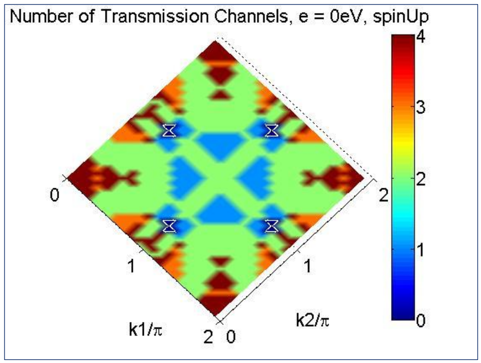
Fig. 6 A plot of the spin up transmission channels \(N_{trc}(E,k_1,k_2)\) in bulk Fe at the Fermi energy (E = 0), versus the transverse momentum \(k_1,k_2\) . Note, all the values of \(N_{trc}(E,k_1,k_2)\) are integers. This shows that there could be up to four spin up channels per unit cell per \(k_1,k_2\) pair for bulk Fe. The symmetry in the plot reflects the crystal symmetry of bulk Fe.

Calculating density of states

As detailed in the Input reference section, density of states (DOS) can be expressed in different ways. In the /examples/Group2_Fe_Bulk/ directory, there is an input file dos.input which essentially has the following lines:

% The input file for the density of states calculation.
% The file NanodcalObject.mat is needed for the calculation.
% type "nanodcal -parameter ? calculation.densityOfStates" for a complete list
% of input parameters which are used for the density of states calculation.
% the hamiltonian of the cNA_LCAO object saved in the file
% NanodcalObject.mat will be used for the calculation.
system.object = NanodcalObject.mat
% Another way to define the hamiltonian is through the input parameter
% system.hamiltonian.
% type "nanodcal -parameter ? system\." for a complete list of input
% parameters which are used to define the system.
% no default value for the calculation name; must be given.
calculation.name = dos
% type "nanodcal -parameter ? calculation.name" for a complete list of
% calculation names.
% some input parameters for the calculation.
calculation.densityOfStates.isIntegrated = true
calculation.densityOfStates.energyRange = [-0.1, 0.1]
calculation.densityOfStates.kSpaceGridNumber = [1 1 1]’*8
calculation.densityOfStates.whatProjected = ’Ell’
calculation.densityOfStates.indexProjected = {0 1 2}
calculation.densityOfStates.whatLocalized = ’Point’
calculation.densityOfStates.regionPosition = [0,0,0]
calculation.densityOfStates.regionVectors = eye(3)*5.2202
calculation.densityOfStates.regionGridNumber = [50 50 1]
calculation.densityOfStates.plot = true
calculation.control.lengthUnit = ang
calculation.control.energyUnit = eV
% type "nanodcal -parameter ? calculation.densityOfStates" for a complete list
% of input parameters which are used for the density of states calculation.

Lines 2-4 tell NanoDCAL to construct DOS from \(E=-5eV\) to \(+5eV\) (Fermi level is shifted at \(E=0\)) using 200 points, and line-4 plots the DOS versus energy. This is the typical DOS plot.

Lines 8-16 were commented out. Suppose we instead comment out lines 3-4 and uncomment lines 8-16, then we would obtain DOS on a real space grid (the local DOS) and integrated over energies. So, line-8 tells NanoDCAL to integrate over \(E\) in a range shown in line-9. How about k? As there is nothing said not to integrate it, k is integrated by default using a k-grid in line-10. But if you wish to resolve the k, you must explicitly specify it by adding a line to the above:

calculation.densityOfStates.isResolved = true

Line-11 tells NanoDCAL to project DOS on orbitals with the given angular momentum specified in line-12. These angular momentum states are called projectors which will appear in the DOS plots. Line-13 tells nanodcal to calculate DOS on real space grid points and lines 14-16 specify the real space region and points. These parameters can take other values, refer to the Input reference section. There are many possible projections of DOS, and some practice is needed to get familiar with them.

Calculating potential

One can inspect the potential terms of the calculated Hamiltonian. In the /examples/Group2_Fe_Bulk/ directory, there is an input file potential.input which essentially has the following lines:

% The input file for the realspace coulomb (delta-hartree) potential.
% The file NanodcalObject.mat is needed for the calculation.
% type "nanodcal -parameter ? calculation.potential" for a complete list
% of input parameters which are used for the potential calculation.
% the realspace potential of the cNA_LCAO object saved in the file
% NanodcalObject.mat will be used for the calculation.
system.object = NanodcalObject.mat
% no default value for the calculation name; must be given.
calculation.name = potential
% type "nanodcal -parameter ? calculation.name" for a complete list of
% calculation names.
% some input parameters for the calculation.
calculation.control.energyUnit = eV
calculation.potential.whatPotential = ’Vdh’
calculation.potential.plot = 1
% type "nanodcal -parameter ? calculation.potential" for a complete list
% of input parameters which are used for the potential calculation.

Line-3 tells NanoDCAL to calculate and plot the Hartree potential \(V_{\delta H}\) which satisfies the following Poisson equation,

(2)\[\nabla^{2}V_{\delta H}=4\pi \left[\rho(\textbf{r})-\rho^{NA}(\textbf{r})\right]\ ,\]

where

(3)\[\rho^{NA}(\textbf{r})={\displaystyle\sum_{I}}\rho^{{NA,I}} (\textbf{r}-\textbf{R}_{I})\]

is the neutral atom density obtained by summing over individual neutral atom densities \(\rho^{{NA,I}}(\textbf{r}-\textbf{R}_{I})\). We refer to Theory section for more details.

By replacing ‘Vdh’ in line-3 with other values, one can calculate and display other terms of the Hamiltonian. Please consulate Input reference for more values.

Calculating charge

One can inspect the charge in the system using the input file charge.input in the /examples/Group2_Fe_Bulk/ directory. This input essentially has the following lines:

% The input file for the analysis on the electronic charge.
% The file NanodcalObject.mat is needed for the calculation.
% type "nanodcal -parameter ? calculation.charge" for a complete list
% of input parameters which are used for the charge calculation.
% the hamiltonian of the cNA_LCAO object saved in the file
% NanodcalObject.mat will be used for the calculation.
system.object = NanodcalObject.mat
% Another way to define the hamiltonian is through the input parameter
% system.hamiltonian.
% type "nanodcal -parameter ? system\." for a complete list of input
% parameters which are used to define the system.
% no default value for the calculation name; must be given.
calculation.name = charge
% type "nanodcal -parameter ? calculation.name" for a complete list of
% calculation names.
% some parameters for the charge analysis
calculation.charge.whatProjected = Ell
calculation.charge.indexProjected = {0 1 2}
% type "nanodcal -parameter ? calculation.charge" for a complete list
% of input parameters which are used for the charge calculation.

Here, line-3 tells NanoDCAL to calculate the number of electrons with the angular momentum specified in line-4, namely project the charge onto the s, p and d states (angular momentum 0, 1 and 2, respectively).

The results are saved in a text file Charge.txt or MAT file Charge.mat. Opening these files, one notices that the spin polarization of the charge is also saved. There are several ways of computing charge information, for instance we may want to know the charge on a particular atom or the total charge of the system. Please go to Input reference section for these and other options.

Summary

While calculation of crystal is important on its own right, for NanoDCAL crystals also serve as electrodes of devices. For quantum transport calculations, a first step is actually determining the electronic structure and properties of the electrodes where crystal calculations must be done. Many other control and system parameters can be set by NanoDCAL so that very flexible calculations of crystal can be done. The Input reference section lists all these possibilities.

[ML08]

Marks, L. D., & Luke, D. R. (2008). Robust mixing for ab initio quantum mechanical calculations. Physical Review B - Condensed Matter and Materials Physics, 78(7), 075114.