Force, Stress, and Structural Relaxation

Using NanoDCAL, atomic forces can be calculated after the self-consistent electronic density is obtained. NanoDCAL also provides decomposition of the force and stress components including terms arising from the kinetic energy, neutral atom interaction, exchange-correlation, and other energy terms. The gradient of the total energy functional with respect to atomic coordinates is taken as the atomic force [Hellmann-Feynman]. Structural relaxation can be performed with the atomic forces. Again, users can find all the input parameters and their default values in the Input reference section. Examples concerning this chapter can be found in the /examples folder of nanodcal.

Forces

In NanoDCAL, atomic force calculation requires the electronic density to be self-consistently calculated first. Afterward, a typical input syntax in the force calculation looks like:

system.object=‘NanodcalObject.mat’
calculation.name = force
calculation.force.movingAtoms = [:math:`a1:b1, a2:b2, ...`]
calculation.force.decomposed = true

Here, the last line controls whether the calculated force is to be separated into different components or not. The ‘movingAtoms’ index on the 3rd line specifies a list of atoms whose forces are to be calculated. The indexing order in the list follows the order in the input atomic file. For instance, consider the AtomBlock - lines 6-21 in the input file Benzene input file. Suppose we wish to compute forces on the first atom, the third, fourth and the fifth atom, and finally the 11th atom, we should specify:

calculation.force.movingAtoms = [:math:`1, 3:5, 11`]

The atomic force calculation can be performed for molecule, bulk or the central region of a multi-probe system. For molecule or bulk systems (Chapters Molecules, Crystals), the force on any atom in the supercell can be calculated. For open structures such as the two-probe, one-probe (Chapters Two Probe Devices, Open Surface Calculations) and multi-probe structures, however, atoms in the buffer layers of the central region but close to the electrodes must be excluded from the force calculation. This is due to physical considerations, i.e. atoms in the buffer layer close to the leads must form the same atomic structure as the leads and as a result, relaxation of these buffer atoms are not allowed. Hence there is no need to compute the atomic forces of these atoms. The situation is schematically shown in Fig. 11. NanoDCAL automatically checks if one is attempting to compute the forces on these buffer atoms that have orbital overlap with the leads and a warning message will be given if this is detected. On the other hand, buffer atoms having no direct orbital overlap with the leads can be relaxed and their forces can therefore be calculated, as shown in Fig. 11.

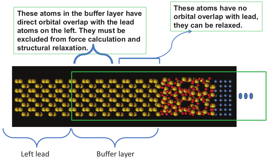
../../_images/2probe-force.png — Fig. 11 Structure of a two probe system where the central region is indicated by the green rectangle. Atoms in the buffer layer of the central region close to the left lead have direct orbital overlap with the lead atoms. These buffer atoms must be excluded in any structural relaxation because they should connect to the leads perfectly, i.e. they should remain as part of the lead even though they sit inside the central region. Other buffer atoms having no orbital overlap with the leads can be relaxed and their forces can be calculated.

The output of the atomic force calculation is the ‘Force.mat’ file in the same folder of the input files.

Stress

The stress tensor of bulk systems can be quite useful. In NanoDCAL, the stress tensor of bulk crystals can be calculated after obtaining the self-consistent electronic density. The syntax looks as follows:

system.object=‘NanodcalObject.mat’
calculation.name = stress
calculation.stress.decomposed = true

In the stress tensor calculation, the atomic forces of all atoms in the supercell are calculated by default and stored in a separate file ( ‘Force.mat’). The third line controls whether the calculated stress is to be separated into different components or not. The output data is stored in the file ‘Stress.mat’ in the input folder.

Structural relaxation

NanoDCAL carries out structural relaxation by damped Newtonian dynamics and/or conjugate gradient (CG) schemes. When the damping is zero, the damped Newtonian dynamics is usually called microcanonical ensemble molecular dynamics or microcanonical molecular dynamics. We shall call the relaxation method of damped Newtonian dynamics as MD in nanodcal.

A relaxation calculation is requested by putting the following lines in the input file:

calculation.name = relaxation
calculation.relaxation.method = MD

or

calculation.relaxation.method = CG

for MD and CG schemes, respectively. In CG, the methods of Polak-Ribi\(\mathrm{\grave{e}}\)re and Fletcher-Reeves can be used:

calculation.relaxation.CG.type = PR

or

calculation.relaxation.CG.type = FR

The equation of motion for the damped-MD relaxation is as follows.

\[\begin{split}\bf{r}_{K}(t_{n+1}) = \bf{r}_{K}(t_{n}) + \Delta\bf{r}_{K}(t_{n})= \bf{r}_{K}(t_{n}) + \bf{v}_{K}(t_{n})\Delta t + \frac{1}{2} \frac{\bf{F}_{K}}{m_K} \Delta t^2\nonumber \\ \bf{v}_{K}(t_{n+1}) = (1-f_{damp}) \bf{v}_{K}(t_{n}) + \frac{\bf{F}_{K}}{m_K}\Delta t\end{split}\]

where subscript \(K\) indicates the atom labelled by \(K\), \(f_{damp}\) is an adjustable damping factor. The time step \(\Delta t\) is updated according to the following rules:

If all the force components \(F_{K,i}\) (\(i=1,2,3\) or \(x,y,z\) etc.) have the same sign as the velocity components \(v_{K,i}\), the time step will increase by a factor \(\alpha\) (\(\alpha = 1.2\) by default).
If more than a third of the force components \(F_{K,i}\) have the opposite sign as velocity components \(v_{K,i}\), the time step will decrease by a factor \(\beta\) (\(\beta = 0.8\) by default), or
If more than a third of the displacement components \(\Delta r_{K,i}\) have reached the upper limit (defined by the parameter calculation.relaxation.MD.maxMove), the time step will decrease by a factor \(\beta\).
If none of the above conditions are met, the time step remains the same.
Clearly, by fixing the control parameters \(\alpha=\beta=1\) (see :ref:`input_ref` section manual), the time step is not updated during the MD relaxation.

The initial time step can be modified by calculation.relaxation.opticalPhononFrequency (see also section1.3.4). The default value is one-fourth of the period of this optical phonon

\[\Delta t_{o} = \frac{1}{4}T_{o} = \frac{\pi}{2} \omega_{o}^{-1}\]

In NanoDCAL, this initial value is absorbed into the mass term, leaving a dimensionless time step, initially set as 1.

Variable supercell

In structural relaxation, there are situations where the supercell changes its shape, for instance under a high external pressure or during a structural phase transformation. These situations require the shape of the calculation supercell to become dynamic variables during the structural relaxation [parrinello-rahman].

By default, the supercell shape does not change in any NanoDCAL calculation. However, the user can relax the supercell shape by using the following control line in the input file:

calculation.relaxation.fixCentralCellShape = false

Note that the relaxation of the shape of supercell is only meaningful for bulk calculations. For open systems such as the two-probe structures, the shape and dimension of the central calculation box are fixed even though the atoms in the central box can be relaxed.

Various constraints can be imposed for relaxing the shape of the supercell.

The volume of the supercell can be fixed, representing an iso-volume transformation. The input syntax is
```
calculation.relaxation.constantVolume = true
```
This default of this condition is false.
External mechanical pressure can be fixed, the input syntax is:
```
calculation.relaxation.constantPressure = [:math:`P_{1}`, ...,
```
\(P_{n}\)] GPa

The unit of pressure can either be GPa of atomic unit (1GPa \(= 3.3989 \times 10^{-5} a.u.\)). The number of the pressure components \(n\) can be 1, 3, 6, or 9, corresponding to uniform pressure \(P=P_{1}\), anisotropic pressure (stress tensor)

(9)\[\begin{split}\sigma = \begin{pmatrix} P_{1} & 0 & 0 \\ 0 & P_{2} & 0 \\ 0 & 0 & P_{3} \end{pmatrix},\end{split}\]

anisotropic pressure plus sheer

(10)\[\begin{split}\sigma = \begin{pmatrix} P_{1} & P_{4} & P_{6} \\ P_{4} & P_{2} & P_{5} \\ P_{6} & P_{5} & P_{3} \end{pmatrix},\end{split}\]

and the most general case

(11)\[\begin{split}\sigma = \begin{pmatrix} P_{1} & P_{4} & P_{7} \\ P_{2} & P_{5} & P_{8} \\ P_{3} & P_{6} & P_{9} \end{pmatrix},\end{split}\]

the last of which is symmetrized internally in the NanoDCAL package. The relaxation process will terminate when the stress tensor of the crystal matches the given value. The default value of the external pressure is zero.
Pre-determined supercell vector variation behavior can be set. This includes several cases. First, one or more supercell vectors can be fixed ( i.e. both directions and lengths). The input syntax is:
```
calculation.relaxation.fixedCellVectors = {:math:`i`}
```
or
```
calculation.relaxation.fixedCellVectors = {:math:`i, j`}
```
where \(i\) and possibly \(j\) are supercell vector indices (1, 2, or 3). The number of indices should be less than three.

Second, the direction of certain supercell vectors can be fixed while their lengths are allowed to relax. The input syntax is:
```
calculation.relaxation.fixedCellDirections = {:math:`i, j,k`}
```
where the specified supercell vectors are listed by their indices. If an index appears both in this constraint and the fixedCellVectors, the latter will be taken.

Sometimes it is convenient to fix the direction of certain supercell vectors and relax their lengths meanwhile keep their lengths to increase or decrease with the same scale. The input syntax is:
```
calculation.relaxation.fixedCellScale = {:math:`i, j,k`}
```
As an example, say we already know the crystal structure of diamond but wish to relax its lattice constant under different external mechanical pressures. For this relaxation, we will set the initial supercell vectors at the equilibrium values of the diamond and put:
```
calculation.relaxation.fixedCellScale = {1, 2, 3}
```
such that the three supercell vectors shall scale at the same rate during the relaxation. The number of indices in the above cell array should be at least two (for ‘same-scaling’ to be meaningful).

The combination of these conditions can produce many new relaxation patterns. For example if we set
```
calculation.relaxation.fixedCellVectors = {1, 2}
calculation.relaxation.constantVolume = true
```
the first two supercell vectors will be fixed while the third can only move horizontally in a plane parallel to the one expanded by the first two vectors.

Since NanoDCAL provides flexibility, mindless input lines may generate conditions that are in conflicts to each other. For instance, if one sets ‘fixedVolume’ and also ‘fixedPressure’, NanoDCAL will give an error message and halt. Combinations of relaxation conditions must be set with extra care to prevent unphysical requirements leading to unpredictable outcome.

Finally, the value of bulk modulus \(B\) is used to control the change rate of cell vectors during supercell relaxation. The change of the cell vectors is given by

(12)\[\epsilon_{n} = \frac{V_{n}}{V_{0}}\frac{\sigma}{3B}\frac{\Delta t_{n}^{2}}{2}\]

where \(V_{n}\) is the volume of the supercell in the \(n^{th}\) relaxation step, \(\sigma\) is the stress tensor (9) and (11). The cell vector of the next relaxation step is given by

\[g_{n+1}=g_{n}(1+\epsilon_{n})\]

where \(g=[\bf{a}_1, \bf{a}_2, \bf{a}_3]\). The input parameter \(B\) has a default value which is rather large, thus the relaxation is typically slow by (12). One can usually find \(B\) for most bulk materials (e.g. diamond, Silicon, etc.). If it is not known, one can test a number of \(B\) values by reducing it, until a proper one is found that gives both fast relaxation and good numerical stability.

Fixed line/plane motion

It is possible to confine some atoms to move on fixed lines or planes. This feature is invoked by the following input syntax:

 calculation.relaxation.constrainGroups1D = {:math:`a1:b1, a2:b2, ...`}
 calculation.relaxation.constrainDirections1D =
{:math:`[e_{1x},e_{1y},e_{1z}], [e_{2x},e_{2y},e_{2z}], ...`}

where the first line defines the groups of atoms moving in lines and the second line defines the line direction of each group. Thus, atoms in the group {\(a1:b1\)} are allowed to move along the line defined by the vector {\([e_{1x},e_{1y},e_{1z}]\)}, etc..

Similarly, for atoms moving in planes, the normal directions of the planes are given and the syntax are like

calculation.relaxation.constrainGroups2D = {:math:`a1:b1, a2:b2, ...`}
calculation.relaxation.constrainDirections2D =
{:math:`[n_{1x},n_{1y},n_{1z}], [n_{2x},n_{2y},n_{2z}], ...`}

where the first line defines the groups of atoms moving in planes and the second line defines the normal direction of each plane. Thus, atoms in the group {\(a1:b1\)} are allowed to move in the plane whose normal vector is {\([n_{1x},n_{1y},n_{1z}]\)}.

Special care must be taken when combining these conditions with the variable supercell options.

Rigid body motion

To relax a large system, one may save some computation time by using the rigid body option of NanoDCAL. In the input file, user can claim a group of atoms to form a ‘rigid body’, i.e. this group of atoms are moved as a whole in the relaxation process during which the bond lengths and bond angles are kept constant. Several rigid bodies can be present simultaneously, as long as they do not share any common atoms. The syntax for setting the rigid body is as follows:

calculation.relaxation.rigidBodies =
{:math:`[i_{1}, ..., i_{m}] , [j_{1}, ..., j_{n}] ...`}

where the \(i's\) and \(j's\) denote the indices of atoms in each rigid body.

Other control parameters

There are several parameters that control the relaxation process. For the MD method (damped Newtonian dynamics), the input line

calculation.relaxation.MD.maxMove = :math:`value`

controls the maximum atomic displacement per atom per step. For small ‘\(value\)’ the relaxation process is more stable but takes more steps to converge.

There is no such constraint for the CG method since it calculates the minimum energy point by performing a line search. The number of line search steps in CG, however, can be limited by

calculation.relaxation.CG.maxLineSearchIterations = :math:`number`

where \(number=2\) is the default. A higher number of line search iterations will result in a more precise lowest energy point along the direction of the line search, but the gain often can not justify the time spent on those extra iteration steps beyond the second. For different systems the optimal number of iterations may vary and the user can tweak this parameter to balance the precision and speed of line search in CG.

There are two parameters that control the length of the time step:

calculation.relaxation.opticalPhononFrequency = :math:`value`
calculation.relaxation.bulkModulus = :math:`value`

The parameter \(opticalPhononFrequency\) is the \(expected\) upper limit of the vibrational frequency of the system. The higher the value, the shorter the time step. If one does not wish to make a guess of this parameter, one can set its value using the following formula: \(\omega_o = \pi/(2\Delta t)\) where \(\Delta t\) is the MD time step (say \(1\) fs). Similarly, the second line above, \(bulkModulus\), serves the same purpose but works on supercell relaxation.

[Hellmann-Feynman]

Hellmann, H (1937). Einführung in die Quantenchemie. Leipzig: Franz Deuticke. p. 285. Feynman, R. P. (1939). “Forces in Molecules”. Physical Review. 56 (4): 340–343.

[parrinello-rahman]

Martonák, R & Laio, A & Parrinello, M. (2003). Predicting Crystal Structures: The Parrinello-Rahman Method Revisited. Physical review letters. 90. 075503.