Molecules
We shall deal with the systems of NanoDCAL as described in Section Systems in NanoDCAL. A system means a specific atomic structure given by atomic positions plus a specification whether it is closed or open. A closed system can be a finite number of atoms enclosed inside a large computation box - called a molecule; or can be a periodic structure consisting of repeating cells along one (1d), two (2d) or three dimensions (3d) - called a crystal. These are familiar configurations in DFT calculation where the computation box or the repeating cell is the supercell. These are referred to as supercell calculations. NanoDCAL also calls the close systems as zero-probe system as in Section Systems in NanoDCAL. The supercell calculations are done like in other DFT electronic packages. This section describes how to carry out a molecule calculation.
Molecular structures
For NanoDCAL, a molecule means a cluster of atoms enclosed inside a supercell, schematically shown in Fig. 4 The goal is to compute the electronic structure and other physical properties of this cluster by DFT.
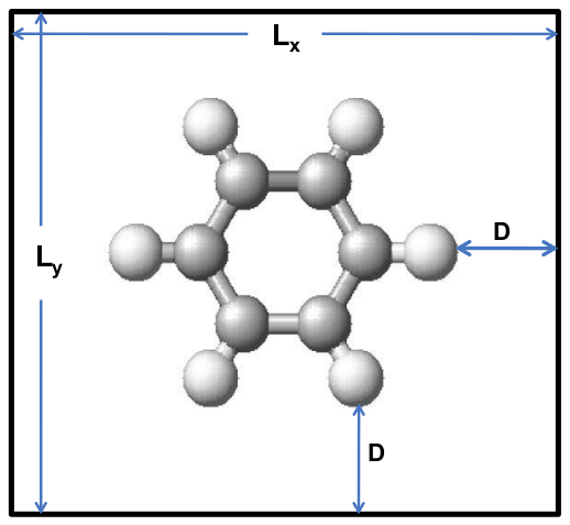
Fig. 4 Schematic plot of a supercell containing a group of atoms. The linear size of the cell is (L x , L y , L z ), and the closest distance from the atoms to the cell boundary is D.
The size \((L_x,L_y,L_z)\) of the supercell must be large enough so that the distance between any atomic core to any boundary of the supercell, \(D\), is greater than the size of any atomic orbital \(\zeta\): \(D > \zeta\). As discussed in Section LCAO basis set and pseudopotentials, in the Theory section as well as in the nanobase User Reference manual, \(\zeta\) is the cutoff radius of neutral atomic orbital (s,p,d). If you use basis functions provided by Nanoacademic (see Section LCAO basis set and pseudopotentials), values of \(\zeta\) for each orbital can be found by clicking the “full” description of the atom database, see Section LCAO basis set and pseudopotentials. It is typically less than ten atomic units (a.u.). Hence a choice of \(D=15\)a.u. should be reasonably safe. However, one should always pay a little attention in choosing \(D\). If you have used nanobase to generate your own basis functions, set your \(D\) larger than your \(\zeta\).
To solve the Kohn-Sham equation for the molecule, boundary conditions on the supercell are needed. If no boundary condition is given in the input file (see below), NanoDCAL automatically uses periodic boundary condition. Since there is a vacuum region between any atom and the supercell boundary (\(D > \zeta\)), images of the atoms due to the periodic boundary condition do not interact. This is the reason to make sure \(D > \zeta\). On the other hand, there are situations where one wishes to apply some boundary conditions for a molecular calculation, for instance calculating electronic structure of a molecular inside a capacitor, i.e. inside an external electric field. For this case you can specify the boundary condition such that a finite voltage difference is set up between two boundaries of the supercell. The default is not to give any boundary condition so that periodic boundary condition at the supercell is applied automatically.
Basic input file
Let’s use the /examples/Group1_C6H6_Molecule/ example to illustrate how
to run NanoDCAL (in the rest of this manual, we shall just specify
this as Group1. Similar specification is applied to other groups of
examples). After starting Matlab, the first task is to copy the
appropriate LCAO basis functions and pseudopotentials of C and H atoms
to the working directory /examples/Group1 or to the /neutralatomdata
subdirectory, from the database /neutralatomdatabase. Section
LCAO basis set and pseudopotentials above discussed how to do this trivially.
Afterward, open the input file scf.input in the /examples/Group1
directory which is shown below
% The input file for the self-consistent field (hamiltonian) calculation.
% The files benzene.xyz, C_DZP.nad, and H_DZP.nad are needed for the calculation.
% type "nanodcal -parameter ? \.SCF\." for a complete list of input parameters
% which are used for the SCF calculation.
% no default value for the calculation name; must be given.
calculation.name = scf
% type "nanodcal -parameter ? calculation.name" for a complete list of
% calculation names.
% default name is empty
system.name = Benzene
% type "nanodcal -parameter ? system\." for a complete list of input
% parameters which are used to define the system.
% default spinType is NoSpin
system.spinType = NoSpin
% centralCellVectors is optional for molecule; nanodcal will choose a suitable
% value for it.
system.centralCellVectors = [14.000,14.000,10.000]
% another possible value of atomCoordinateFormat is fractional.
% default value is cartesian
system.atomCoordinateFormat = cartesian
% this parameter defines the atoms of the system through a file. Another
% way to define the atoms is through the parameter atomBlock
system.atomFile = benzene.xyz
% default value of atomPositionShift is [0 0 0]
system.atomPositionShift = [3.4510, 4.4280, 3.0];
% the position of the atoms, which are defined in the file benzene.xyz, will
% be shift according to the value of atomPositionShift.
% default value of atomPositionPrecision is 1e-3 bohr
system.atomPositionPrecision = 1e-2
% the precision of the position used in symmetry analysis
% default value of orbitalType is AtomicData
system.orbitalType = DZP
% default value of the Type is LDA_PZ81
calculation.xcFunctional.Type = LDA_PZ81
% type "nanodcal -parameter ? xcFunctional\." for a complete list of input
% parameters which are used to define the exchange-correlation functional.
% the length unit used for the input and output.
% default value is Angstrom
calculation.control.lengthUnit = Angstrom
% type "nanodcal -parameter ? control\." for a complete list of input control
% parameters.
% the length unit used for the input and output.
% default value is eV
calculation.control.energyUnit = eV
% the length unit used for the input and output.
% default value is Degree
calculation.control.angleUnit = Degree
% control the output in the log.txt file;
% the larger the number, the more the output.
calculation.control.logOutputLevel = [1,2]
% control the output of the files of the calculated results;
% the larger the number, the more the files.
calculation.control.txtResultsOutputLevel = 7
calculation.SCF.mixingMode = ’H’
% type "nanodcal -parameter ? \.SCF\." for a complete list of input parameters
% which are used for the SCF calculation.
In Benzene input file, Line-3 begins with system.centralCellVectors which is a keyWord having values of (\(L_x,L_y,L_z\)) in atomic units (1a.u. length = 0.529 angstrom). Thus, the supercell in this example is a cubic box with linear sizes (15,15,15). Lines 4 and 5 are commented out, but they indicate another method of setting up (\(L_x,L_y,L_z\)).
Line-7 has a keyWord system.atomBlock which specifies the number of
atoms N in the system, N = 12 in our example here. This is a block of
data which begins with line-7 and ends at line-21. Inside this block,
line-8 is a header whose first four entries must be (not necessarily in
order) AtomType, X, Y, Z. There can be other entries such as spin, which
we will discuss later. The values of (X, Y, Z) are the position of an
atom in the system. The value of AtomType is the symbol of the atomic
specie that is located at (X, Y, Z), i.e. the prefix of file names of
the basis functions to be used in the present calculation. For example,
in /neutralatomdata you can see a file with a name C_DZP.mat or
H_DZP.mat etc., thus if you use these input files, you must specify
AtomType to be C or H, etc. Another header must be given is
OrbitalType which describes what kind of atomic orbital is used in the
basis set. It is normally SZ, SZP, DZ, DZP, etc. In general, larger
basis set gives more accurate result but requires more computational
time. DZP is a reasonable compromise between accuracy and computational
speed. Some practice is necessary to understand what kind of basis is
best suitable for your research problem.
Nanobase allows you to generate various
basis functions if they are not in the provided database. For instance,
suppose there is a need to use TZP—triple \(\zeta\) polarized
orbital for a particular atom in the atomBlock of
Benzene input file, and a C_TZP.nad has been
generated by nanobase. You can specify
the OrbitalType for this atom as TZP in the atom list of
Benzene input file. In other words, the
OrbitalType does not have to be the same for all the atoms. Finally, the
basis database is generated with certain exchange-correlation (XC)
functionals such as the LDA and GGA, as specified in the database. Users
can generate them by other XC potentials using the
nanobase.
When you copied the basis data file for a calculation, it is helpful to
write down in a notebook what basis has been copied, for future
references. At the end of any calculation, the information about basis
functions are saved in a text output file named Atoms.txt. All the
calculation results and input details are also saved in the output file
cNA_LCAO_Object.mat which is a MAT file (see below).
While AtomType and OrbitalType could be any string, the database of the
corresponding neutral atom in /neutralatomdata must be named as
AtomType_OrbitalType.mat, (e.g. H_DZP.mat or Cu_SZP.mat etc.) and
located in the current directory or in the /neutralatomdata directory.
The file in the current directory has higher priority. As discussed
above, the OrbitalType of each individual atom can be specified
differently, i.e. any atom can have its own unique basis different from
other atoms. This can be done even if atoms are of the same AtomType.
However, if all atoms have the same OrbitalType, then the OrbitalType
can be specified elsewhere in the input file scf.input using a kewWord
system.orbitalType. For example, a line:
system.orbitalType = DZP
tells NanoDCAL to use DZP for all the atoms. In this case, one does not need to write ‘DZP’ following each atom in the AtomBlock. The OrbitalType following each atom in the AtomBlock has higher priority.
Lines 9-20 of Benzene input file specify the coordinates of the 12 atoms of this molecule. Finally, line-21 ends the data block. In NanoDCAL, the origin of the coordinate system is fixed at (0,0,0). In this example, the supercell extends from (0,0,0) to (15,15,15). The best practice is to prepare positions of the atoms so that they are all enclosed inside the supercell. For our example, since all the coordinates of the 12 atoms are positive and less than 15, they are all enclosed inside the supercell. Nevertheless, NanoDCAL will work even if the molecule (or part of it) sits outside the supercell, but we do not recommend it because it does not look nice and can become confusing later on.
The atomBlock (the coordinates of the atoms) can also be put into a
separate file and included into the scf.input. This way, your
scf.input avoids being clogged by many lines of numerical data. In the
/examples/Group1 subdirectory, you can find another control file
scf1.input and the atomic position file benzene.xyz. scf1.input is the
same as scf.input, except that the atomBlock (lines 7-21 of
Benzene input file)
is replaced by the following line:
system.atomFile = benzene.xyz
With this keyWord, the coordinates of the atoms are put into a separate
file benzene.xyz. Please open this xyz file and find its format.
Finally, since we use DZP for all the atoms, we now specify this fact in
scf1.input. Hence in the benzene.xyz, the OrbitalType on each line can
be removed without causing problems.
The last line of Benzene input file (line 22) informs NanoDCAL to carry out a SCF run, which is to calculate the self-consistent field or the Hamiltonian of the molecule. Since this is a closed system, the SCF is just the conventional DFT self-consistent iteration. The keyWords calculation.name can have many values, such as transmission, IVCurve, DOS, etc. Refer to the Input reference section for all the values.
Basic standard output
The extent of the output is controlled by the following input parameter:
calculation.control.logOutputLevel
Please see Input reference section for this output control. In the rest of this section, we discuss the default output.
Let’s run NanoDCAL with the /examples/Group1 example by typing the
following inside the command window of Matlab:
nanodcal scf.input
Many lines of output appear in the command window, see Benzene output. These lines is also saved in the log.txt file. The standard output are grouped into several blocks and they are self-explanatory. Here, lines 1-17 give system summary; lines 18-29 calculates atomic potentials from neutral atom data; lines 30-46 calculates the self-consistent potentials.
System Summary:
System Name: NoName
System Type: molecule, no spin
System Symmetry: D6
# of Atoms in Central Cell: 12
# of Electrons of Central Cell Atoms: 30
# of Basis of Central Cell Atoms: 108
Parameters Summary:
XC functional type: LDA_PZ81
central cell base vectors:
v1 = (1.500000e+001, 0.000000e+000, 0.000000e+000)
v2 = (0.000000e+000, 1.500000e+001, 0.000000e+000)
v3 = (0.000000e+000, 0.000000e+000, 1.500000e+001)
realspace grid numbers: [90 90 90]
realspace grid volume: 0.0046296 Angstrom3̂
k-space grid numbers: [1 1 1]
electronic temperature: 100 K
calculation of the rigid atomic field ......
calculating S, T, and Vnl ...... :: finished. time used:  000:00:02.26
calculating Vna ...... :: finished. time used: 000:00:03.81
calculating Rpc ....... :: finished. time used: 000:00:00.04
calculating Rna & initial Rho ...... :: finished. time used: 000:00:01.42
calculating real space XC potential ...... :: finished. time used: 000:00:01.61
calculating real space Veff ...... :: finished. time used: 000:00:00.24
constructing static part of H ...... :: finished. time used: 000:00:00.09
calculating Veff Matrix ...... :: finished. time used: 000:00:02.36
constructing Hamiltonian ...... :: finished. time used: 000:00:00.03
---- calculation of rigidAtomicField finished. time used: 000:00:11.93
calculation of the self-consistent field ......
Some parameters used:
The calculation is starting from hamiltonian matrix.
The physical quantity to be mixed is hamiltonian matrix.
The mixing is performed by class cMixerBroyden.
Self-Consistent Loops:
Loop # time hMatrix rhoMatrix bandEnergy gridCharge orbitalCharge
1 000:00:08.26 -1.9788E-001 0.0000E+000 -3.6471E+002 2.8839E-004 -1.0658E-014
2 000:00:07.74 4.5429E-001 5.2083E-003 -5.7991E+000 2.9013E-004 2.1316E-014
3 000:00:07.53 7.8082E-002 1.3108E-002 1.1158E+000 2.9409E-004 -7.1054E-014
4 000:00:07.46 5.5167E-001 1.1990E-003 1.0535E+001 2.9408E-004 -1.5277E-013
5 000:00:07.48 9.7128E-002 8.7044E-003 1.8212E+000 2.9342E-004 7.1054E-015
6 000:00:07.54 2.5231E-003 1.5202E-003 3.9389E-002 2.9330E-004 1.1013E-013
7 000:00:07.37 1.2600E-002 -1.2155E-004 2.1811E-001 2.9329E-004 -1.2434E-013
8 000:00:07.39 8.9478E-004 -6.8097E-004 1.7644E-002 2.9326E-004 -5.3291E-014
9 000:00:07.59 -2.1326E-004 -2.1305E-005 -1.4711E-003 2.9326E-004 1.7764E-014
---- calculation of the self-consistent field finished. total energy = -1023.2281.
time used: 000:01:14.09
saving calculated results ...... :: finished. time used: 000:00:04.07
---- ---- ---- All the calculations have been finished. time used: 000:01:32.62
Line-2 says the system has not been given a name, so NoName. One may wish to give a name to this system by adding a line
system.name = benzene
inside scf.input anywhere outside the atomic data block. After re-run,
line-2 of Benzene output becomes System Name: benzene.
 System Summary:
 System Name: NoName
 System Type: molecule, no spin
 System Symmetry: D6
 # of Atoms in Central Cell: 12
 # of Electrons of Central Cell Atoms: 30
 # of Basis of Central Cell Atoms: 108
 Parameters Summary:
 XC functional type: LDA_PZ81
 central cell base vectors:
 v1 = (1.500000e+001, 0.000000e+000, 0.000000e+000)
 v2 = (0.000000e+000, 1.500000e+001, 0.000000e+000)
 v3 = (0.000000e+000, 0.000000e+000, 1.500000e+001)
 realspace grid numbers: [90 90 90]
 realspace grid volume: 0.0046296 Angstrom3̂
 k-space grid numbers: [1 1 1]
 electronic temperature: 100 K
 calculation of the rigid atomic field ......
 calculating S, T, and Vnl ...... :: finished. time used: 000:00:02.26
 calculating Vna ...... :: finished. time used: 000:00:03.81
 calculating Rpc ....... :: finished. time used: 000:00:00.04
 calculating Rna & initial Rho ...... :: finished. time used: 000:00:01.42
 calculating real space XC potential ...... :: finished. time used: 000:00:01.61
 calculating real space Veff ...... :: finished. time used: 000:00:00.24
 constructing static part of H ...... :: finished. time used: 000:00:00.09
 calculating Veff Matrix ...... :: finished. time used: 000:00:02.36
 constructing Hamiltonian ...... :: finished. time used: 000:00:00.03
 —— calculation of rigidAtomicField finished. time used: 000:00:11.93
 calculation of the self-consistent field ......
 Some parameters used:
 The calculation is starting from hamiltonian matrix.
 The physical quantity to be mixed is hamiltonian matrix.
 The mixing is performed by class cMixerBroyden.
 Self-Consistent Loops:
 Loop # time hMatrix rhoMatrix bandEnergy gridCharge orbitalCharge
 1 000:00:08.26 -1.9788E-001 0.0000E+000 -3.6471E+002 2.8839E-004
-1.0658E-014
 2 000:00:07.74 4.5429E-001 5.2083E-003 -5.7991E+000 2.9013E-004
2.1316E-014
 3 000:00:07.53 7.8082E-002 1.3108E-002 1.1158E+000 2.9409E-004
-7.1054E-014
 4 000:00:07.46 5.5167E-001 1.1990E-003 1.0535E+001 2.9408E-004
-1.5277E-013
 5 000:00:07.48 9.7128E-002 8.7044E-003 1.8212E+000 2.9342E-004
7.1054E-015
 6 000:00:07.54 2.5231E-003 1.5202E-003 3.9389E-002 2.9330E-004
1.1013E-013
 7 000:00:07.37 1.2600E-002 -1.2155E-004 2.1811E-001 2.9329E-004
-1.2434E-013
 8 000:00:07.39 8.9478E-004 -6.8097E-004 1.7644E-002 2.9326E-004
-5.3291E-014
 9 000:00:07.59 -2.1326E-004 -2.1305E-005 -1.4711E-003 2.9326E-004
1.7764E-014
 —— calculation of the self-consistent field finished. total energy =
-1023.2281. time used: 000:01:14.09
 saving calculated results ...... :: finished. time used: 000:00:04.07
 —— —— —— All the calculations have been finished. time used: 000:01:32.62
Line-3 is important: it states that we are computing a molecular system
without worrying about spin. How does NanoDCAL figure out it is a
molecule rather than a periodic system? This is because we have
correctly set supercell sizes in scf.input such that \(D > \zeta\)
(see discussions in section Molecular structures). Now, suppose we
made a mistake in scf.input by using:
system.centralCellVectors = [8 15 15]
instead of the line-3 of Benzene input file, namely we put a smaller \(L_x = 8\) such that \(D < \zeta\). In this case, NanoDCAL will still run and give results, but line-3 of Benzene output would become: “System Type: periodic-1D, no spin”. Hence, instead of a molecule, NanoDCAL treats it as an one-dimensional periodic system because we have (mistakenly) specified \(D < \zeta\). There is no error on the part of NanoDCAL because if we specify \(D < \zeta\), we have told NanoDCAL that the \(\zeta\)-functions extend to outside the supercell. When this happens, NanoDCAL naturally thinks that there are other supercells neighboring the original one and the system is therefore a periodic structure along the connected supercells. By reading line-3, one can immediately see what kind of system has been computed.
Line-3 also specifies that there is no spin involved in this calculation. In general, NanoDCAL allows users to specify spin polarized calculation by using a keyWord system.spinType. There are several spin resolved computation capabilities as specified by the following keyValues,
system.spinType = NoSpin

system.spinType = CollinearSpin

system.spinType = GeneralSpin
The default spinType is NoSpin which was used in this /examples/Group1
example. For other spin types, please refer to Section
Spin Polarized Calculation and Spintronics
Line-4 indicates the symmetry group of the input atomic structure, D6 for the benzene molecule here. This is not terribly useful for a small molecule calculation, but it is helpful for periodic systems which will be discussed in Crystals Lines 5-6 states that there are 12 atoms and total of 30 electrons in the supercell. Line-7 indicates that 108 basis functions are used for this calculation. For a H atom, DZP means two s-orbital plus a p-polarization orbital, i.e. five orbital per H. There are six H atoms making a total of 30 orbital. For a C atom, DZP means two s-orbital and two p-orbital - eight s, p orbital plus a d-polarization orbital, thus 13 per C. There are six C atoms making 78 orbital. Hence the total number of basis functions is 108.
Lines 8-17 in the output (Benzene output) is a
parameter summary. Line-9 specifies the exchange-correlation functional
that has been used, e.g. LDA_PZ81 - the local density functional
approximation (LDA) of Purdew-Zunger form [PZ81]. The
XC functionals can be changed by using the following keyWord:
calculation.xcFunctional.Type = keyValue
where keyValue can various LDA or GGA functional. Refer to Input reference for all possibilities. Importantly, users can supply their own XC functional using the NanoDCAL API, also described in the Input reference section.
Line-14 gives real-space grid numbers: [90, 90, 90]. This means that the supercell specified in the scf.input has been meshed by a real-space grid of \(90\) points in each of the three dimensions. Where do these numbers come from? Because the real-space grid has not been specified in scf.input, NanoDCAL did the discretization automatically using a default. This default method uses an upper energy cutoff \(E_{cutoff}\) to decide the grid number \(N\) by the following formula:
where \(L\) is the linear length of the supercell. The default values of \(E_{cutoff}\) are 20, 50, or 150 Hartree, depending on the value of another control parameter whose default value is ‘normal’:
calculation.control.precision = low, normal, or high
These precision parameters tell NanoDCAL what numerical accuracy should be enforced. Using the normal precision \(E_{cutoff}=50\) Hartree, (1) gives \(N=90\) for our example and a real space grid volume of 0.0046296Å\(^3\), as indicated in line-15 of Benzene output. This volume is simply \(\delta x \delta y \delta z\) for a cubic grid.
However, the real-space grid number can be specified by users, for instance:
calculation.realspacegrids.number = [60 80 128]’
Putting this line into scf.input will set real-space grid numbers to
[60,80,128] and over-rides the default. What grid to use depends on the
research problem and should be tested, but a discretization of
\(\delta x \approx 0.3\) a.u. should be a rough compromise to start
which allows us to roughly set \(N \sim L/\delta
x\).
Line-16 presents the k-space grid size: [1 1 1]. Any “molecule” is a finite system involving a finite number of atoms. No k-sampling is necessary so that only one k-value, \(\bf{k}=0\), is used in the k-sampling. But for periodic systems, the k-space grid is in general not just one point. See Section Basic standard output for more details on periodic systems.
Line-17 says electronic temperature is \(100\) Kelvin. This is the default used in the Fermi function for periodic or molecule calculations. Its value can be changed by a keyWord, e.g.
calculation.occupationFunction.temperature = 50
Although temperature is a physical quantity, here it is used to stabilize numerical calculations in DFT. If temperature is put to zero in a periodic calculation, the DFT self-consistent iteration can have difficulty to converge due to slight variations of the Fermi level from one iteration step to the next. This is because in periodic calculations, the Fermi level is varied to guarantee charge neutrality of the supercell. The same is true for molecule calculations where the supercell containing the molecule Fig. 4 is periodically extended in all directions. The problem does not occur in transport calculations where the Fermi level is set by the device electrodes.
The next block in the Benzene output presents the actual calculation process in NanoDCAL. We begin by the calculation of the “rigid atomic field” in lines 18-28: these are overlap matrix \(S\), kinetic energy matrix \(T\), nonlocal pseudopotential matrix \(V_{nl}\), neutral atom potential matrix \(V_{na}\), some quantities related to the radial wave functions of the LCAO basis sets \(R_{pc}\) (partial core charge density) and \(R_{na}\) (neutral atom charge density). Other quantities are also calculated by using \(R_{na}\), namely charge density \(\rho\), Hartree potential \(V_H\), the exchange-correlation (XC) potential \(V_{XC}\), and the effective potential \(V_{eff}\):
The definitions of these quantities are given in the Theory.
Concerning initialization: the default is to initialize \(\rho\) to
the neutral atom density - by summing up densities of isolated neutral
atoms in the system. You can also tell NanoDCAL to initialize to
other initial density or initial physical quantities. For instance, you
can initialize the charge density by your own data using the control
parameter calculation.SCF.donatorObject: please read
Input reference for more details. Initializing density differently than
the default can be useful for two-probe calculations, see
Two Probe Devices for further discussions. For
molecule and periodic calculations, the default usually works fine. The
matrix elements of relevant quantities appearing in the above list are
defined in the Theory section.
Finally, we arrive at the DFT iterative calculation of the self-consistent field, lines 29-46. Line-31 indicates that the self-consistent calculation starts from the initial Hamiltonian matrix - the default. But there are situations we may want to start from other quantities such as an initial charge density. The following keyWord sets how a calculation should start:
calculation.SCF.startingMode = H, or mRho, or realRho
If ‘mRho’, calculation starts from an initial density matrix; if ‘realRho’, it start from a real space density. Refer to Input reference for more discussions.
Line-32 indicates that the physical quantity to be mixed from one iteration step to the next is the Hamiltonian matrix, which is the default. Again, we can mix different quantities by using the following keyWord:
calculation.SCF.mixingMode = H, or mRho, or realRho
Line-33 indicates that the mixing method used by NanoDCAL in the self-consistent iteration is the class cMixerBroyden, i.e. using the Broyden mixing method [J88]. It is actually the default mixer. There are other mixing methods specified by the following:
calculation.SCF.mixer = cMixerBroyden/cMixerLinearor/...
Importantly, many calculation methods in nanodcal are plug-in calculators that can be easily replaced by users. Refer to Input reference for more discussions. For information, type:
nanodcal -help plug-in
nanodcal -api
In particular, the mixers of NanoDCAL are plug-in calculators. The mixer calculator is a structure with two fields: ‘class’ and ‘parameter’. We thus can set:
calculation.SCF.mixer.class = cMixerBroyden
calculation.SCF.mixer.parameter.beta = 1e-3
Lines 34-45 outputs the actual self-consistent DFT iteration process. It took nine iterations to reach the default self-consistency. The quantities being monitored are summarized in Table 4. These quantities are the difference between the present iteration step and the last iteration step. When the monitored quantity is a matrix such as H matrix and \(\rho\) matrix, the values indicate the largest difference amongst all the matrix elements.
NanoDCAL stops when the calculation reaches self-consistency specified by default or by the user. One can change the self-consistency criterion by monitoring different physical quantities using the following keyWord:
calculation.SCF.monitoredVariableName = ...
where ‘…’ is a name list which is a cell array of strings, these strings are summarized in the 2nd column of Table 4. The default value of this keyWord is the cell (hMatrix, rhoMatrix, bandEnergy, gridCharge, orbitalCharge). A user can create his own monitor for NanoDCAL to follow, for example, he may wish to use the convergence of total magnetic moment as the self-consistency criterion. Therefore, if there is any user-defined name among the name list, the corresponding calculator must be specified as:
calculation.SCF.monitoredVariableCalculator = ...
How to construct a user supplied calculator is a high level function of NanoDCAL and we refer to the Input reference section. For now, let’s just stick with the supplied monitors in Table 4.
Monitored quantity |
Meaning |
|
|---|---|---|
1 |
hMatrix |
Hamiltonian matrix element |
2 |
rhoMatrix |
Density matrix element |
3 |
bandEnergy |
Band structure energy of system |
4 |
gridCharge |
Charge difference by real space grid |
5 |
orbitalCharge |
Charge difference by orbital |
6 |
spinPolar |
total spin polarization |
7 |
subTotalEnergy |
Energy excluding nucleus-nucleus contribution |
8 |
totalEnergy |
Total energy of system |
9 |
realSpaceRho |
\(\rho(i,j,k)\) on real space grid point (i,j,k) |
10 |
realSpaceVdh |
\(V_{\delta H}(i,j,k)\) on real space grid point (i,j,k) |
11 |
realSpaceVeff |
\(V_{eff}(i,j,k)\) on real space grid point (i,j,k) |
Output data files
In the previous sections we focused on the standard output showing up on the computer screen. NanoDCAL can actually provide all sorts of data stored on hard-drive for later analysis. In the Section entitled “Control parameters for the calculation” in the Input reference section manual, one can find keyWords for controlling the level of outputs from a nanodcal run.
The most essential output files are shown in Table 5, which are automatically generated in each NanoDCAL run. In Table 5, the first four files are Hamiltonian and density matrix data in both MAT and ASCII format. Entry 5 is the MAT-file containing all the calculated results, an example will be given in Section Calculating band structure below. Entry 6 is an object that contains all information of the calculation and it is the most essential output that is used for calculating other physical quantities. To retrieve information, type:
load cNA_LCAO_Object.mat
object
...
Summary
In this Section we have outlined how to carry out a basic
pseudopotential based equilibrium DFT calculation for an isolated
cluster of atoms. We used the /examples/Group1 example for our
discussion. There are many other examples in the /example directory to
illustrate the usage of NanoDCAL. Please also consult
Input reference for all the possible input options. In
the next Section, we present the calculation for periodic structures.
Output file name |
Information stored |
File type |
|
|---|---|---|---|
1 |
Hamiltonian.mat |
Hamiltonian matrix |
mat |
2 |
Hamiltonian.txt |
Hamiltonian matrix |
ascii |
3 |
DensityMatrix.mat |
Density matrix |
mat |
4 |
DensityMatrix.txt |
Density matrix |
ascii |
5 |
CalculatedResults.mat |
All calculated results |
mat |
6 |
NanodcalObject.mat |
Everything |
object |
7 |
\(\cdots\) |
Perdew, J. P., & Zunger, A. (1981). Self-interaction correction to density-functional approximations for many-electron systems. Physical Review B, 23(10), 5048–5079.
Johnson, D. D. (1988). Modified Broydens method for accelerating convergence in self-consistent calculations. Physical Review B, 38(18), 12807–12813.