6. Josephson-energy solver
This section explains the theory behind the quantum-transport framework used in the
Josephson-energy Solver.
Introduction
Superconducting circuits are among the most promising platforms for scalable quantum computing. Fundamental to widely used devices based on transmons are Al/AlOx/Al Josephson junctions shunted by a large capacitance. As the energy spectrum is weakly anharmonic, the first two levels of these devices can be used as a computational basis for quantum computing. In this picture, the qubit transition frequency, the difference between these two energy levels, is set primarily by the Josephson energy \(E_{\text{J}}\), associated with the Josephson junction, and charging energy \(E_{C}\), associated with the shunting capacitance [BGGW21].
Solving practical quantum problems may require \(10^{5}\) to \(10^{7}\) noisy qubits. This makes device-to-device variability a major challenge for the calibration and the tuning of such large systems. Many factors contribute to device-to-device variability. At the top of the list, we have the variability of the Josephson energy, which is related to the critical current \(I_{\text{c}}\) by
where \(\hbar\) is the reduced Planck constant and \(\mathrm{e}\) is the elementary charge.
The large variability of the Josephson energy arises from the fact that Josephson junctions operate in the tunneling regime and the critical current \(I_{\text{c}}\) depends exponentially on microscopic barrier details. These details include local Al/AlOx thickness fluctuations, effective barrier height variations and even contamination atoms.
QTCAD® offers a module to compute the variability of \(E_{\text{J}}\)
induced by Al/AlOx interface roughness based on the quantum-mechanical
modelling framework of [ZBG26].
The module comprises the interface-roughness model class
GaussianRandomField, a
Solver and a
SolverParams class to store
parameters specific to the solver.
Below, we present a summary of the interface-roughness and quantum-transport models that comprise the theoretical framework.
Interface roughness model
Let us consider the interfaces between the aluminum (Al) leads and a thin dielectric
layer of aluminium oxide (AlOx) of a Josephson junction.
We assume the dielectric layer to have a rectangular transverse section, with side
lengths \(l_x\) and \(l_y\), and ideal thickness \(d\).
We will model the roughness of these interfaces as a Gaussian random field
(GaussianRandomField)
with a specialized power spectral density.
Let us denote the interface height by \(h\left(x,y\right)\), where \(x\) and \(y\) are the transverse coordinates, with the transport direction being along \(z\). We also assume that
and the following two-point correlation function
where \(\sigma\) is the root-mean-square (RMS) value of the interface height along the transport direction and \(\xi\) is the transverse correlation length.
Given \(\sigma\) and \(\xi\), rough interfaces can be generated by filtering white noise in Fourier space using the corresponding power spectral density (the Fourier transform of the correlation function) and applying an inverse Fourier transform to the result. One example of the two generated rough interfaces of a given junction is shown in Fig. 6.1.
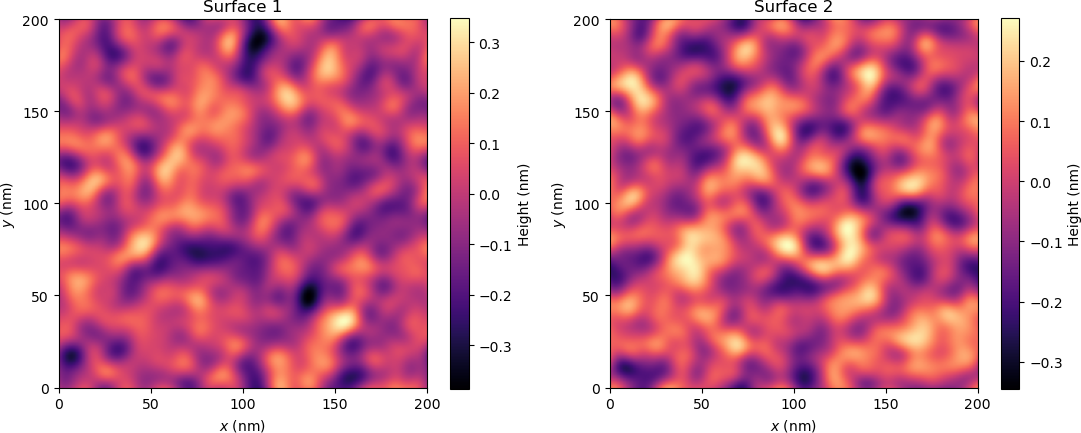
Fig. 6.1 Intensity plots representing the roughness profile of the two interfaces of a square Josephson junction with side lengths \(l_x = l_y = 200\) nm. The height variation was obtained using Gaussian random fields with the same parameters \(\sigma\) and \(\xi\) on each interface.
We remark the following on \(\xi\) and \(\sigma\), which are required to
instantiate
GaussianRandomField:
The transverse correlation length \(\xi\) is set by the characteristic lateral length scale of microstructural features in the Al leads. The most notable feature is the Al grain size that imprint thickness variations onto the AlOx barrier [ZBG26].
In Al/AlOx/Al tunnel-junction stacks characterized by transmission electron microscopy (TEM), the Al electrodes are commonly observed to be polycrystalline with columnar grains on the order of a few tens of nanometers [FRS+19, NKZ+16].
The RMS height \(\sigma\) is set by the vertical amplitude of thickness fluctuations, primarily controlled by the Al surface roughness and oxidation/growth non-uniformity.
This roughness model therefore describes deviations of the two dielectric–metal interfaces from their ideal case, in which they are separated by the nominal dielectric thickness \(d\). Furthermore, we assume \(\sigma\) and \(\xi\) to be identical for the two Al/AlOx interfaces of the Josephson junctions. The resulting local barrier thickness is obtained by adding the two interface height profiles to the nominal thickness \(d\), thus defining the spatially varying tunnel-barrier profile used in the transport calculation.
Quantum-transport model
Let us now connect the roughness-induced barrier geometry to the Josephson energy. Fundamentally, in a Josephson junction, the critical current of a Josephson junction \(I_{\text{c}}\) can be calculated by solving the Bogoliubov–de Gennes (BdG) equation
where
is the single-particle Hamiltonian, with the potential energy being given by
\(V(\mathbf{r}) = e U_{\text{barrier}}(\mathbf{r})\), where
\(U_{\text{barrier}}\) represents the electrostatic potential profile of a
three-dimensional rectangular tunnel barrier.
Also, \(E_{\text{F}}\) is the Fermi energy, \(m\) is the electron mass,
\(\Delta\left( \mathbf{r}\right)\) is the superconducting pair potential
(SolverParams.sc_gap),
\(u\left(\mathbf{r}\right)\) and \(v\left( \mathbf{r}\right)\) are the electron-
and hole-like components of the quasi-particle wave function.
However, solving the BdG equation directly for a realistic Josephson junction is extremely challenging. A typical junction transport region has dimensions of \(100\) nm \(\times\) \(100\) nm \(\times\) \(1\) nm, whereas the real-space grid spacing must be on the order of \(1\) Å to resolve electronic wave functions with a Fermi wave length of \(\lambda_{\text{F}} \approx 3.6\) Å (for bulk Al). This would require a three-dimensional grid of approximately \(10^{3}\times10^{3}\times10\) points, making a direct real-space BdG calculation computationally expensive.
To tackle the computational challenge, as in [ZBG26], we adopt two approximations to simplify the transport model in QTCAD®. The first approximation is to use the Ambegaokar–Baratoff (AB) relation
Here, \(R_{\text{N}}\) is the normal-state resistance. Its calculation is simpler than obtaining \(I_{\text{c}}\) via the BdG equation because it only requires an evaluation of the transmission coefficient at the Fermi energy rather than an integration over the entire energy range. Furthermore, the system size is reduced by half, since only the electron-like quasi-particles need to be considered.
Note
The use of the AB relation was justified in [ZBG26], where a comparison between \(I_{\text{c}}\) computed using the BdG equation and the AB formula for a rectangular tunnel barrier shows an excellent agreement over a wide range of junction thicknesses. This can be seen in Fig. 2 of [ZBG26] and the associated discussion.
The second approximation is the local thickness approximation, where we separate the transport direction from the transverse directions. Transverse coupling in a junction is negligible because it operates in the tunneling regime. Hence, transport is predominantly governed by the local barrier profile along the transport direction.
We therefore partition the junction into a large ensemble
of \(n\) locally uniform and independent subsystems (tunnel barriers or channels;
SolverParams.n_partitions)
parallel in the transverse plane. The total normal-state conductance \(\propto
1/R_{\text{N}}\) is then approximated as the sum of the conductances of these subsystems.
To be precise, we consider rectangular junctions of nominal thickness \(d \in [0.1,
3]\) nm and side lengths \(l_{x}\) and \(l_{y}\), partitioned along each
respective direction in \(n_{x}\) and \(n_{y}\) subsystems.
Next, the conductance is computed for each of the partitioned junctions of side lengths
\(l_{x}/n_{x}\) and \(l_{y}/n_{y}\).
The total normal-state conductance is then obtained by summing these subsystems’
conductances, which, in the continuum limit, would be an integral of the conductance
density over the transverse coordinates.
Finally, \(E_{\text{J}}\) is obtained from the AB relation.
Also, we consider the junctions as two free-electron metallic leads separated by the
rectangular tunnel barrier of height \(U_{\text{barrier}}\)
(SolverParams.potential_barrier_height)
and width \(d + h(x,y)\).
When instantiating the Josephson-energy
Solver, in addition to
pre-configured
GaussianRandomField and
SolverParams objects, the
thickness \(d\) should be passed. Also, the side lengths can be either passed
directly or extracted from a provided layout OAS/GDS file.
Note
This local thickness approximation is justified by noting that, for the usual range of parameters involved, the change of the tunnel-barrier thickness over a lateral distance \(\lambda _{\text{F}}\) is
where \(\lambda_{\text{d}} = 1/\sqrt{2mU_{\text{barrier}}/\hbar ^{2}}\) is the wave function decaying length in the tunnel barrier, with \(U_{\text{barrier}}\) being the effective tunnel barrier height of the Al/AlOx interface. Such an approximation remains valid for a conservative range of \(U_{\text{barrier}} \in [0.1, 3]\) eV and the likely ratios \(\sigma/\xi\) from experiments.
Statistics of variability-study results
When computing the variability of \(E_{\text{J}}\) using the Gaussian random field
described above, the resulting distribution of \(E_{\text{J}}\)
(Solver.energy_distribution)
will not be Gaussian-like, but skewed toward larger values.
We can readily understand that by noting that the effective tunnel barrier width is
normally distributed. Therefore, since \(E_{\text{J}}\) has an exponential
dependence on the tunnel barrier width, the distribution of \(E_{\text{J}}\) will
follow a log-normal distribution.
The corresponding probability density function is
where \(\mu_{\text{J}}\) and \(\sigma_{\text{J}}\) are the mean and standard
deviation of \(\log(E_{\text{J}})\). Then, the mean
(Solver.mean_value) and
variance of \(E_{\text{J}}\) respectively are
and
from which the standard deviation can be trivially obtained
(Solver.std_deviation).
These expressions show why the distribution of \(E_{\text{J}}\) over a large
ensemble of Josephson junctions
(SolverParams.n_samples)
becomes increasingly skewed and broadened as the underlying fluctuations grow.