AI-relaxer (CHGNet) tutorial
Requirements
Software components
nanotools
Briefing
Here comes the Artificial Intelligence-driven (AI) relaxer for two-probe systems! This guide will walk you through the process step by step.
In atomistic modeling and simulation, “relax” refers to the process of allowing the atoms or molecules of the system to adjust their positions and configurations in order to reach a state of minimal energy or equilibrium.
Why is it necessary to relax the central region of a two-probe transport system? The central region plays a crucial role in determining transport properties such as carrier current and conductance. These properties are sensitive to the atomic structure of the central region; even some relatively small structural changes can significantly impact the results. Therefore, structural relaxation in the central region is essential for obtaining reliable transport properties.
Why use this relaxer when traditional DFT relaxation methods are available? While traditional DFT relaxation methods are powerful and reliable, they are also computationally expensive. Relaxations for systems with a few hundred to a few thousand atoms using traditional DFT can take anywhere from minutes to several hours or even days, depending on factors such as computational resources, software efficiency, system size, convergence criteria, chosen methodology, and the quality of initial guesses. To strike a balance between accuracy and efficiency, a method that is both fast and reasonably accurate is desired. CHGNet [1] is a pretrained universal neural network potential for charge-informed atomistic modeling, which is specifically designed to accurately predict atomic forces and energies for atomistic simulations. One can use CHGNet to relax a system with several hundreds or even thousands of atoms very efficiently, often in just a few minutes based on our tests.
The AI-relaxer facilitates the structure relaxation process using the Atomic Simulation Environment (ASE) [2] and the pretrained CHGNet force model. After relaxation, the relaxed atomic structure is saved for further use. One can also plot the total energy of the central region of the two-probe device during the structural optimization and visualize the relaxation trajectory. The AI-relaxer significantly enhances the efficiency of two-probe device simulations.
Scripts
from nanotools.utils import ureg
from nanotools import AtomCell
from nanotools.relaxation.two_probe import NBRelaxer

left = AtomCell(positions=("ni_graphene.xyz","bohr"), avec=[[4.64682193271677,0.0,0.0],[0.0,8.04853168139326,0.0],[0.0,0.0,30.27076472739540]]* ureg.bohr)
right = AtomCell(positions=("graphene.xyz","bohr"), avec=[[4.64682193271677,0.0,0.0],[0.0,8.04853168139326,0.0],[0.0,0.0,30.27076472739540]]* ureg.bohr)
center = AtomCell(positions=("ni_graphene_center.xyz","bohr"), avec=[[4.64682193271677,0.0,0.0],[0.0,48.29119008835956,0.0],[0.0,0.0,30.27076472739540]]* ureg.bohr)

relaxer = NBRelaxer(left, right, center, transport_axis="Y")
relaxer.relax()
relaxer.write(filename="graphene_armchair_relaxed", output_format="vasp")
relaxer.plot_energy(filename="graphene_armchair_Energy", show=True)
relaxer.visualize_trajectory()
Explanations
This example demonstrates a graphene spintronic system [3], which includes an armchair-graphene/Nickel central region and two semi-infinite leads: armchair-graphene and armchair-graphene-Nickel.
In this script, we import the NBRelaxer class from the nanotools.relaxation.two_probe module.
In this context, NB stands for “Nano Builder”. The NBRelaxer class is used to relax the material system using the CHGNet potential.
After importing the necessary modules, the first step is to create the central region and leads using the AtomCell object.
The positions parameter must be provided. If positions specifies the path of an xyz file, the formula parameter is automatically read from the xyz file.
However, if positions does not specify an xyz file, formula must be used to define the chemical formula, as shown in the following example:
right = AtomCell(formula="C4",
positions=([
   [1.16170546635838, 3.35586034069663, 16.96215117189000],
   [1.16170546635838, 0.67290534069663, 16.96711717189000],
   [3.48511646635838, 7.38012834069663, 16.96215117189000],
   [3.48511646635838, 4.69717334069663, 16.96711717189000]],"bohr"),
avec=[[4.64682193271677, 0.0, 0.0], [0.0, 8.04853168139326, 0.0], [0.0, 0.0, 30.27076472739540]]* ureg.bohr)
The avec parameter is used to define the lattice vectors. If the unit is not specified, the default unit is angstrom.
The next step involves creating the NBRelaxer object, which is used to relax the central region of a two-probe system.
relaxer = NBRelaxer(left, right, center, tolerance=0.01, max_steps=50, transport_axis="Y")
The NBRelaxer object takes the AtomCell objects of the central region and leads as inputs.
The tolerance parameter refers to the maximum force allowed on atoms during relaxation,
with a default value of 0.05 eV/angstrom. The max_steps parameter sets the maximum number of steps
for relaxation, which is set to 100 by default. The transport_axis parameter determines
the transport direction, which defaults to “Z”. The tolerance, max_steps, and transport_axis
parameters are optional and can be omitted if the default values are acceptable.
The nanotools.relaxation.two_probe.relax() method initiates the relaxation process for the central region.
Upon invocation, it first verifies that enough buffer atoms on the sides of the central region are fixed during the relaxation process.
To clarify, when we say “enough,” we mean that the number of buffer atoms on each side of the central region must be
no less than the number of atoms present in both the left and right leads. Subsequently, the method sets up the CHGNet calculator
and initiates the relaxation process using the BFGS minimizer from the ASE package.
The relaxation process is terminated when the maximum number of steps is reached or
the force on all atoms is below the specified tolerance.
The nanotools.relaxation.two_probe.write() method is used to write the relaxed structure to a file in a specified format.
It supports a variety of formats, including “vasp”, “xyz”, and “cif”, among others.
If no format is specified, the method defaults to exporting in the “xyz” format.
The filename parameter is optional. If it’s not provided, the method will use “relaxed”
as the default filename for the output file.
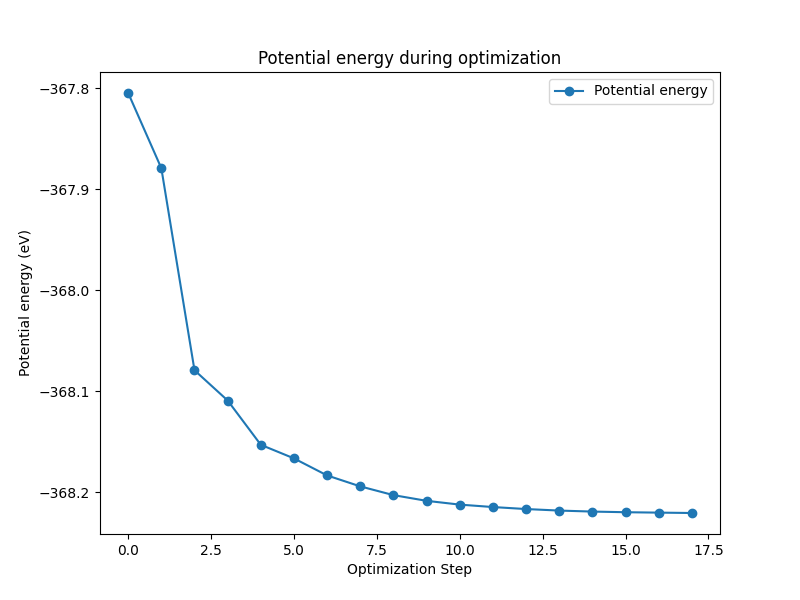
The nanotools.relaxation.two_probe.plot_energy() method is used to plot the potential energy during the optimization process and save it to a file.
You could decide whether to show the plot by setting the show parameter to True or False.
The filename parameter is optional. If it’s not provided, the method will use “Potential energy” as the default filename for the output file.
When we plot the potential energy in this case, we can see that the energy decreases as the optimization progresses:
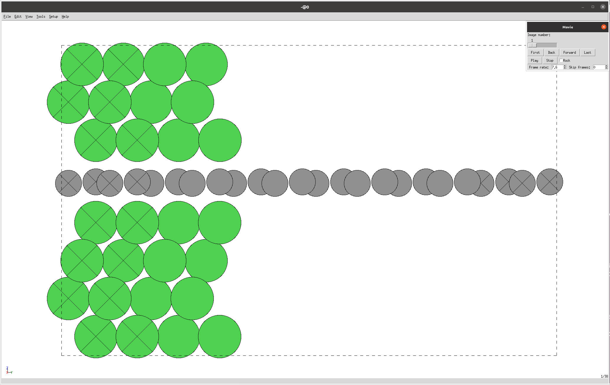
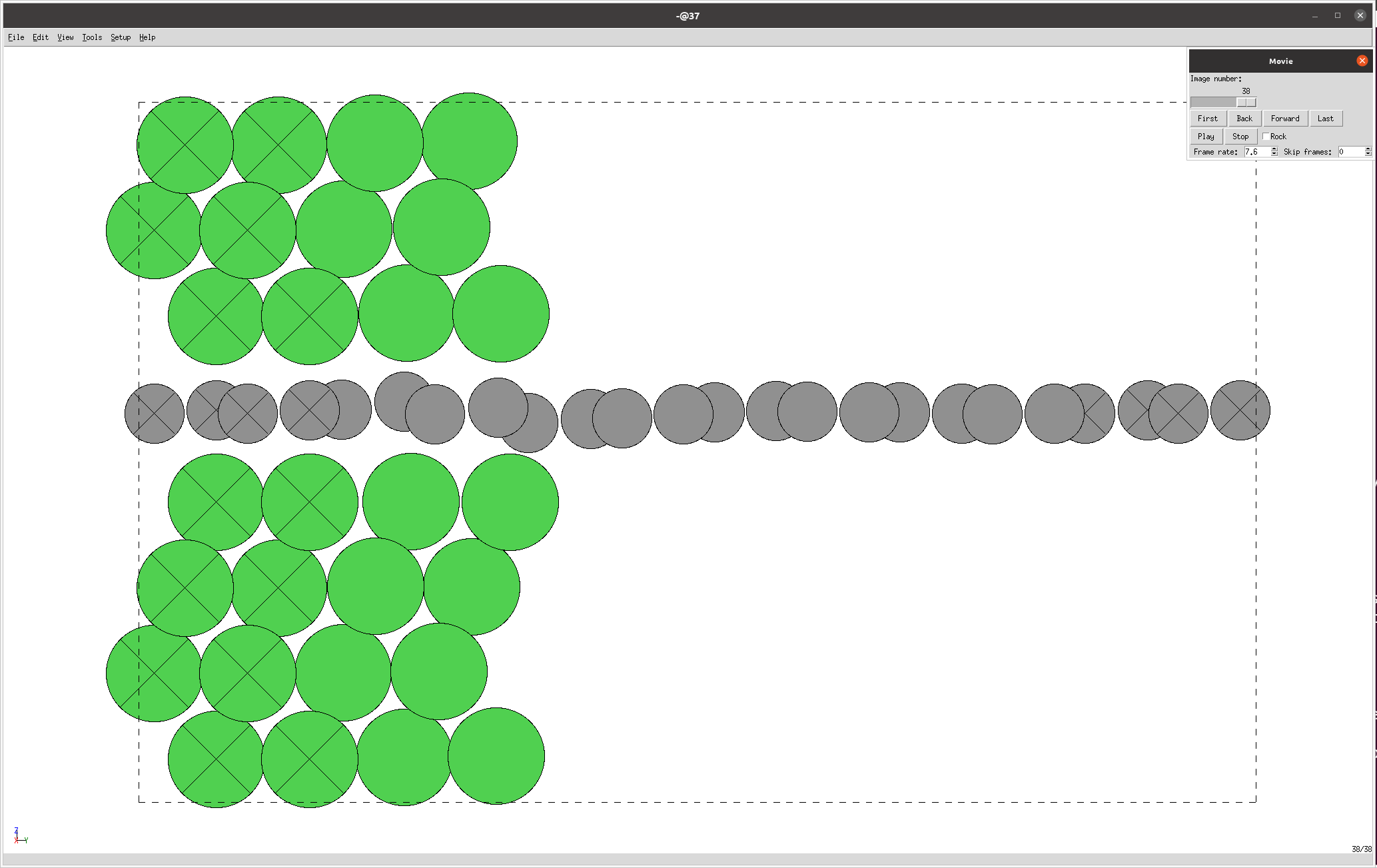
The nanotools.relaxation.two_probe.visualize_trajectory() method is used to visualize the trajectory of the relaxation process.
In this case, the trajectory is visualized using the ASE GUI, which displays the structure at each step (the crossed atoms are “fixed”):