Transmission tutorial

Requirements

Software components

• nanotools

• NanoDCAL+

Pseudopotentials

• C_AtomicData.mat

Copy the mat file from the pseudo database to the current working directory and export NANODCALPLUS_PSEUDO=$PWD.

Briefing

This tutorial presents a minimal example of transmission calculation for a two-probe transport system. The system to be addressed is a crystalline carbon nano-tube (CNT).

Setup

python script

from nanotools import Atoms, Cell, Species, System, TotalEnergy, Transmission, TwoProbe
import numpy as np

cell = Cell(avec=[[20.0, 0.0, 0.0], [0.0, 20.0, 0.0], [0.0 , 0.0 , 2.4595]], resolution=0.2)
atoms= Atoms(positions="cnt.xyz")
sys = System(cell=cell, atoms=atoms)
sys.kpoint.set_grid([1,1,50])
center = TotalEnergy(sys)
left = center
right= center

dev = TwoProbe(left=left, center=center, right=right, transport_axis=2)
dev.center.solver.set_mpi_command("mpiexec -n 4")
# dev.center.solver.mpidist.zptprc=4
dev.solve()

cal = Transmission.from_twoprobe(twoprb=dev)
cal.solve(energies = np.linspace(-5, 5, num=101))
cal.plot(filename="cnt_transm.png", show=True)

structure file cnt.xyz, in Cartesian coordinates

12
CNT
C 8.08866505    10.69566903     0.61487804
C 8.44186547    11.30743011     1.84462196
C 9.64679958    12.00309914     1.84462196
C 10.35320042   12.00309914     0.61487804
C 11.55813453   11.30743011     0.61487804
C 11.91133495   10.69566903     1.84462196
C 11.91133495   9.30433097      1.84462196
C 11.55813453   8.69256989      0.61487804
C 10.35320042   7.99690086      0.61487804
C 9.64679958    7.99690086      1.84462196
C 8.44186547    8.69256989      1.84462196
C 8.08866505    9.30433097      0.61487804

Explanations

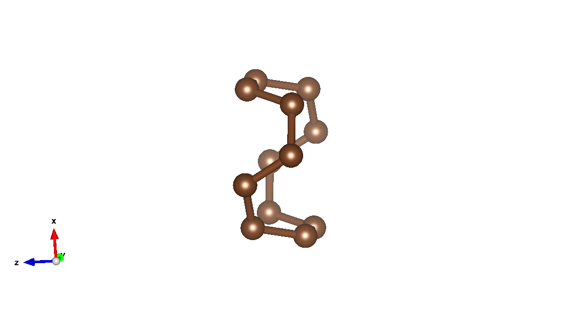
As sketched in the above diagram, a two-probe transport system consists of three sub-systems, corresponding to the two electrical leads and a quantum scattering structure in between. The leads are regarded as in thermal equilibrium and therefore can be resolved with the basic DFT calculator under periodic boundary conditions. The remaining task is solving the quantum scattering problem with lead electronic structures taken as boundary conditions. We shall first perform a self-consistent calculation for our CNT structure, and then compute the very important quantity, transmission, which indicates the maximum possible electric current at a given energy level.

System definition

The following code section describes a unit cell of an armchair carbon nano-tube (see figure above)

cell = Cell(avec=[[20.0, 0.0, 0.0], [0.0, 20.0, 0.0], [0.0 , 0.0 , 2.4595]], resolution=0.2)
atoms= Atoms(positions="cnt.xyz")
sys = System(cell=cell, atoms=atoms)

A grid of reciprocal (k) points is also needed for the periodic calculation of lead structures. This is specified by

sys.kpoint.set_grid([1,1,50])

We set only one k-point in the transversal plane since there is vacuum buffer all around the nanotube. Along the transport direction, on the other hand, a sufficient number of k-points should be used since lead structures are periodic. In general, only one k-grid needs be specified for the whole two-probe calculation: k-points along the transport dimension are automatically removed when it comes to the NEGF calculation for the central region.

The sys object is then used to initialize a TotalEnergy calculator (see tutorial_etot.md)

center = TotalEnergy(sys)

The TwoProbe calculator, which manages the work-flow of self-consistent calculations, can be initialized as

left = center
right= center
dev = TwoProbe(left=left, center=center, right=right, transport_axis=2)

where left, center, and right are TotalEnergy calculators for the respective sub-systems. In this tutorial, the three sub-systems are structually identical. Therefore, we simply assign the same calculator twice

Since it happens quite often that a few or all of the sub-systems in a two-probe system share the same structure, nanotools provides a simplified interface for this case

dev = TwoProbe(center=center, transport_axis=2)

Now left and right are assumed identical to center. When only right is omitted, eg.

dev = TwoProbe(left=left, center=center, transport_axis=2)

right is assumed identical to left.

Nevertheless, note that one must explicitly specify the transport_axis parameter (along which dimension transport occurs) in defining a TwoProbe calculator. In the current example, transport_axis=2 corresponds to the z-dimension (remember that python uses 0-based indexing).

Self-consistent calculation

We then launch the self-consistent calculation by typing in

dev.center.solver.set_mpi_command("mpiexec -n 4")
dev.center.solver.mpidist.zptprc=4
dev.solve()

The first two lines set mpi-related parameters to accelerate the calculation. Here we assign 4 processors. The zptprc parameter indicates the number of energy points at which Green functions are computed in parallel. This parameter is better to be maximized for small simulation tasks.

Upon executing dev.solve(), a few json files will appear in the directory; they are left.json, right.json, and nano_2prb_in.json. In many cases the leads may be structurally identical; if so, right.json will be omitted. Self-consistent calculations are first carried out for leads, using the rescuplus executable, with left.json or right.json as its input files. The outputs are written in left_out.json, left_out.h5, right_out.json and right_out.h5. After the lead calculations are finished, nanodcalplus will be executed with nano_2prb_in.json as its input file. nanodcalplus performs the self-consistent calculation for the quantum scattering problem, and the results will be saved in nano_2prb_out.json and center_out.h5. Note that center_out.h5 contains charge densities and potentials only of the central scattering region. All the workflow described here is managed by dev.solve().

One may restart a two-probe calculation based on an existing charge-density file, e.g.

...
dev.center.solver.restart.densityPath = "center_out.h5"
dev.solve()

Transmission

The self-consistent calculation must precedes the transmission calculation, since the latter requires existing ground-state density data, i.e. _out.h5 files.

The Transmission calculator is dedicated to the transmission computation. In our case, we can simply create such a calculator from the existing TwoProbe object and use its solve method to launch the calculation.

cal = Transmission.from_twoprobe(twoprb=dev)
cal.solve(energies = np.linspace(-5, 5, num=101))

Finally, we visualize the transmission profile by typing in

cal.plot(filename="cnt_transm.png", show=True)

You should see something similar to

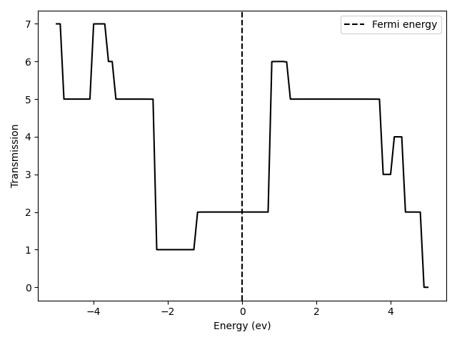
Since we are simulating a perfectly intrinsic carbon nano-tube, its transmission profile shows a step-wise shape. The integer transmission value at each step simply equals the band degeneracy.