Photo-current tutorial

Requirements

Software components

nanotools
NanoDCAL+

Pseudopotentials

C_LDA_TM_DZP.mat

Copy the mat file from the pseudo database to the current working directory and export NANODCALPLUS_PSEUDO=$PWD.

Theory

According to the first order perturbation theory, the charge current moving into a lead $L$ induced by optical excitation is calculated as

\[ J_L = \frac{ieN}{h} \int \textup{Tr} \Gamma_L(E) (1-f_L(E)) G^r(E) M G^<(E-\hbar \omega) M^\dagger G^a(E) + \textup{Tr} \Gamma_L(E) f_L(E) G^r(E) M^\dagger G^>(E+\hbar \omega) M G^a(E) dE \]

where $N$ is number of photons, $\Gamma$ is broadening function of the lead, $f$ is Fermi-Dirac function, $G$ is Green function, and $M$ is the matrix form of the polarization operator

\[ \hat{M} = \frac{e}{m_0} \sqrt{\frac{\hbar}{ 2 \omega \epsilon_r \epsilon_0 V}} \mathbf{\hat{e} \cdot \hat{p}} \]

Here $\omega$ is the light frequency, $\epsilon_r\epsilon_0$ is permitivity of the material, $V$ is volume of the optical cavity, $\hat{p}$ is quantum momentum operator, and $\mathbf{\hat{e}}$ is a complex polarization vector defined with an orthonormal pair of real vectors $\mathbf{(e_1,e_2)}$ and a pair of elliptical angles $(\theta,\phi)$:

\[ \mathbf{\hat{e}} = [\cos (\theta) \cos (\phi) - i \sin (\theta) \sin(\phi)]\mathbf{{e_1}} +[\sin(\theta) \cos (\phi)+ i \cos(\theta) \sin(\phi)]\mathbf{{e_2}} \]

To simplify the workflow of computing $J_L$, we define the dimensionless photo-transmission as follows

\[ \mathfrak{T}_L(E) = \left ( \frac{\alpha c h a_0^2}{i \hbar \omega \epsilon_r V} \right )^{-1} \textup{Tr} [ \Gamma_L(E) (1-f_L(E)) G^r(E) M G^<(E-\hbar \omega) M^\dagger G^a(E) + \Gamma_L(E) f_L(E) G^r(E) M^\dagger G^>(E+\hbar \omega) M G^a(E) ] \]

where $c$ is vacuum speed of light, $a_0$ is Bohr radius, $\alpha$ is fine-structure constant. We further define the dimensionless photocurrent response coefficient

\[ \mathfrak{R}_L = \frac{\alpha}{\hbar \omega} \int \mathfrak{T}_L(E) dE \]

Hence the photocurrent can be expressed as

\[ J*L = e a_0^2 \sqrt{\mu_r/\epsilon_r } I*\omega \mathfrak{R}\_L \]

where $I_\omega$ is the photon-flux in terms of particle density:

\[ I_\omega=\frac{N}{V}\frac{c}{\sqrt{\epsilon_r \mu_r}} \]

For experimentalists, it may be more convenient to characterize photon-flux with the energy-flux parameter $P_\omega$, i.e. optical power per area, which has a simple relation with $I_\omega$: $P_\omega = \hbar \omega I_\omega$.

Example

In this example, we calculate the photo-current through an electrically biased carbon chain. Note that there should exist a charge current through the chain even without optical field. Here the photo-current refers to the part of charge-current specifically induced by optical excitation.

python script

from nanotools.photocurrent import PhotoCurrent
from nanotools import Atoms, Cell, System, TotalEnergy, TwoProbe
from nanotools.utils import ureg
import numpy as np

cell = Cell(avec=[12, 0.0, 0.0,
                  0.0, 12, 0.0,
                  0.0, 0.0, 16],
                  resolution = 0.12)
atoms= Atoms(positions="c8.xyz")
sys = System(cell=cell, atoms=atoms)
sys.kpoint.set_grid([1,1,40])
sys.pop.set_type("fd")
sys.pop.set_sigma(0.01)
center = TotalEnergy(sys)

# define the two-probe ground-state problem and solve
dev = TwoProbe(center=center, bias=0.5, transport_axis=2)
dev.set_mpi_command(mpi=f"mpiexec -n 4")
dev.left.solver.mpidist.kptprc = 4 # parallelize over k points
dev.left.solver.restart.densityPath = "left_out.h5"
dev.center.solver.restart.densityPath = "center_out.h5"
# dev.center.solver.mpidist.zptprc = 4 # parallelize over contour energy points
dev.solve()

#define the orthonormal basis vectors
base_vec = [  [-0.118915679855830, 0.316904693970085, -0.940973153721270],
              [-0.857210947821695, 0.445467497858298, 0.258356535211516] ]

#define the photo-current problem and solve
sct = PhotoCurrent.from_twoprobe(dev,
      polar_basis_vec = base_vec,
      theta = np.pi/2, phi= np.pi/4,
      elec_energy_resol = 0.01, #energy resolution for photo-transmission (the integrand)
      photon_energy = 0.7)
sct.solve()
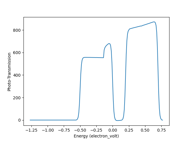
sct.plot_photo_transmission(lead="left", save_to="phot_left.json")
sct.plot_photo_transmission(lead="right", save_to="phot_right.json")
r = sct.get_response()
c = sct.get_photo_current(
    flux=1.0 * ureg.watt / ureg.meter**2, # optical energy flux
    mu=1.0, epsilon=1.0) # relative material permitivity and permeability
print("photo-current response coefficient:")
print(r)
print("photo-current (density):")
print(c)

structure file c8.xyz, in Cartesian coordinates

8
s x y z
C     6.00000000      6.00000000      1
C     6.00000000      6.00000000      3
C     6.00000000      6.00000000      5
C     6.00000000      6.00000000      7
C     6.00000000      6.00000000      9
C     6.00000000      6.00000000      11
C     6.00000000      6.00000000      13
C     6.00000000      6.00000000      15

On your screen, you should see the following output when the program is finished

photo-current response coefficient:
[[[-14.87261766  14.87272017]]]
photo-current (density):
[[[-0.041317034921601804 0.04131731971157402]]] ampere / meter ** 2

Both response and current are 3d-arrays, with each dimension corresponding to photon-energy, spin, and lead. In this example, the optical mode is assumed monocolor, and spin is degenerate. Therefore, the output for photo-current here should be interpreted as $J_L = -0.041317 A / m^2 \: J_R = 0.041317 A / m^2$. The current (density) unit is $A / m^2$ because we apply periodic boundary condition across the transversal directions of the device structure. The charge current through one single carbon chain should be calculated as $J_{L/R}$ multiplied by the cross section area of the simulation cell.

In addition, the following figure should appear in your work directory. This figure plots $\mathfrak{T}_R$ as a function of electronic energies.

Photo-transmission