Scattering states tutorial

Requirements

Software components

• nanotools

• NanoDCAL+

Pseudopotentials

• C_LDA_TM_DZP.mat

Copy the mat file from the pseudo database to the current working directory and export NANODCALPLUS_PSEUDO=$PWD.

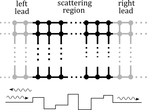
Fig. 1 A two-probe transport system

Briefing

Scattering states are eigenstates of a quantum transport system. Given an incident wave from one lead of the device, we wish to compute its scattering rates into other outgoing waves at the same energy level, together with the scattered wave amplitude in the center of the device. To be concrete, the program solves the following linear system of equations [1]

\[\begin{split}\begin{bmatrix} h_{11} - \Sigma_{L} & h_{12} & & & \\ h_{21} & h_{22} & & 0 & \\ & & \ddots & & \\ & 0 & & h_{n-1,n-1} & h_{n-1,n} \\ & & & h_{n,n-1} & h_{nn} - \Sigma_{R} \end{bmatrix} \begin{bmatrix} \phi_1\\ \\ \vdots \\ \\ \phi_n \end{bmatrix}= \begin{bmatrix} S\\ 0\\ \vdots \\ \\ 0 \end{bmatrix}\end{split}\]

where \Sigma represents lead self-energies, S is a source term arising from incident waves, and the solution to this equation, i.e. \phi_1 \cdots \phi_n, are coefficients of the scattered wavefunction. The reflection and the transmission coefficients are then calculated from the following equations [2]

\[ \begin{align}\begin{aligned}\mathbf{r} = [\mathbf{\Phi}_L^-]^{-1} [\phi_1 - \phi_1^+]\\\mathbf{t} = [\mathbf{\Phi}_R^+]^{-1} \phi_n\end{aligned}\end{align} \]

since the reflected and the transmitted waves must be linear combinations of outgoing waves in the leads, whose coefficients are put as matrix-columns in \mathbf{\Phi}_L^- and \mathbf{\Phi}_R^+.

This tutorial demonstrates the computational workflow by analyzing a carbon chain system with an anti-parallel spin configuration in the leads.

Scripts

left.py

from nanotools import Atoms, Cell, System, TotalEnergy

with open("left.xyz", "w") as f:
     f.write(
"""3
s x y z sz
C     6.00000000      6.00000000      7.25000000      0.5
C     6.00000000      6.00000000      4.35000000      0.5
C     6.0             6.00000000      1.45000000      0.5
""")

npc = 4
cell = Cell(avec=[12, 0.0, 0.0,
                  0.0, 12, 0.0,
                  0.0 , 0.0 , 8.7],
                  grid =[92, 92, 68])
atoms= Atoms(positions="left.xyz")
sys = System(cell=cell, atoms=atoms)
sys.hamiltonian.ispin = 2
sys.atoms.set_initial_magnetic_moments("left.xyz")
sys.kpoint.set_grid([1,1,100])
sys.pop.type = "fd"
sys.pop.set_sigma(0.01)
etot = TotalEnergy(sys)
etot.solver.mpidist.kptprc = npc
etot.solver.cmd.mpi = f"mpiexec -n {npc}"
etot.solver.restart.densityPath = "left_out.h5"
etot.solve(input="left", output="left_out")

right.py

from nanotools import Atoms, Cell, System, TotalEnergy

with open("right.xyz", "w") as f:
     f.write(
"""3
s x y z sz
C     6.00000000      6.00000000      7.25000000      -0.5
C     6.00000000      6.00000000      4.35000000      -0.5
C     6.0             6.00000000      1.45000000      -0.5
""")

npc = 4
cell = Cell(avec=[12, 0.0, 0.0,
                  0.0, 12, 0.0,
                  0.0 , 0.0 , 8.7],
                  grid =[92, 92, 68])
atoms= Atoms(positions="right.xyz")
sys = System(cell=cell, atoms=atoms)
sys.hamiltonian.ispin = 2
sys.atoms.set_initial_magnetic_moments("right.xyz")
sys.kpoint.set_grid([1,1,100])
sys.pop.type = "fd"
sys.pop.set_sigma(0.01)
etot = TotalEnergy(sys)
etot.solver.mpidist.kptprc = npc
etot.solver.cmd.mpi = f"mpiexec -n {npc}"
etot.solver.restart.densityPath = "right_out.h5"
etot.solve(input="right", output="right_out")

center.py

from nanotools import Atoms, Cell, System, TotalEnergy, Transmission, TwoProbe
import numpy as np

with open("center.xyz", "w") as f:
     f.write(
"""12
s x y z sz
C   6.00000000      6.00000000      33.35000000     1.5
C   6.00000000      6.00000000      24.65000000     1.5
C   6.00000000      6.00000000      15.95000000     1.5
C   6.00000000      6.00000000      7.25000000      1.5
C   6.00000000      6.00000000      30.45000000     1.5
C   6.00000000      6.00000000      21.75000000     1.5
C   6.00000000      6.00000000      13.05000000     1.5
C   6.00000000      6.00000000      4.35000000      1.5
C   6.00000000      6.00000000      27.55000000     1.5
C   6.00000000      6.00000000      18.850000       1.5
C   6.00000000      6.00000000      10.15000000     1.5
C   6.00000000      6.00000000      1.45000000      1.5
""")

left = TotalEnergy.read(filename="left_out.json")
right= TotalEnergy.read(filename="right_out.json")

cell = Cell(avec=[12, 0.0, 0.0,
                  0.0, 12, 0.0,
                  0.0 , 0.0 , 34.8],
            grid=[92, 92, 272])
atoms= Atoms(positions="center.xyz")
sys = System(cell=cell, atoms=atoms)
sys.hamiltonian.ispin = 2
sys.atoms.set_initial_magnetic_moments("center.xyz")
sys.kpoint.set_grid([1,1,1])
sys.pop.type = "fd"
sys.pop.sigma= 0.01
sys.pop.nPole= 20
center = TotalEnergy(sys)

npc = 8
dev = TwoProbe(left=left, center=center, right=right, transport_axis=2)
dev.center.solver.cmd.mpi = f"mpiexec -n {npc}"
dev.center.solver.mix.alpha = 0.1
dev.center.solver.restart.densityPath = "center_out.h5"
dev.center.solver.mix.precond = "kerker"
# dev.center.solver.mpidist.zptprc = npc
dev.center.solver.mix.maxit = 100
dev.solve()

transm.py

import numpy as np
from nanotools import TwoProbe, Transmission
dev = TwoProbe.read(filename="nano_2prb_out.json")
trs = Transmission.from_twoprobe(twoprb=dev)
trs.solve(energies = np.linspace(0, 1.6, num=200))
trs.plot(filename="transm.png")

scatt.py

from nanotools import TwoProbe
from nanotools.scattering import ScatteringStates
dev = TwoProbe.read(filename="nano_2prb_out.json")
dev.center.system.kpoint.set_fractional_coordinates([[0,0,0]])
sct = ScatteringStates.from_twoprobe(dev)
sct.solve(energy=1.2) # compute scattering states at 1.2eV

analy.py

from nanotools import ScatteringStates
calc = ScatteringStates.read("nano_scatt_in.json")
incoming= calc.get_bloch(lead="left", direction="in", k_long_index=0)
outgoing= calc.get_bloch(lead="right", direction="out", k_long_index=0)
t = abs(calc.get_scatter_rate(incoming, outgoing))**2  # t=0.302
calc.plot_isosurfaces(**incoming, vals=[1.])
wave = calc.get_scatt_wave(**incoming)

Explanations

The physical system consists of a chain of carbon atoms with equal distances. We divide the chain into three regions, i.e. left, center, and right. We start with the ground-state calculation for left lead by running left.py, where the spin polarization is set upward. Next we run right.py for the right lead, with downward spin. After getting the ground states for leads, we proceed with the two probe calculation by running center.py. To gain a general understanding of the transport properties of our device, we compute its transmission using transm.py. The result is presented in the following figure.

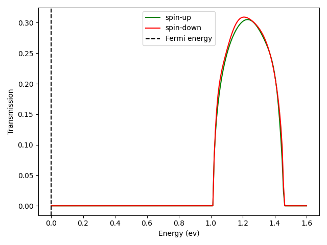
Fig. 2 Transmission profile of carbon chain

We then compute the scattering states (scatt.py) at the energy level 1.2eV. The result is saved in nano_scatt_out.h5 file, which contains information about incoming and outgoing waves in both leads, their scattering rates, and corresponding wave-functions in the central scattering region of the device. To ease access to the data, we have implemented a few methods in the ScatteringStates class. The following script extracts information on a pair of incoming/outgoing Bloch-waves hosted by the left and the right leads respectively.

from nanotools import ScatteringStates
calc = ScatteringStates.read("nano_scatt_in.json")
incoming = calc.get_bloch(lead="left", direction="in", k_long_index=0)
outgoing = calc.get_bloch(lead="right", direction="out", k_long_index=0)

The get_bloch method returns a dictionary for incoming:

{'lead': 'left',
 'direction': 'in',
 'spin': 1,
 'spin_direction': 'up',
 'k_trans_frac': array([0, 0, 0]),
 'k_trans_index': 0,
 'k_long_index': 0,
 'k_long_frac': -0.25836461407263456,
 'energy': 1.2,
 'energy_index': 0
 }

Note that there can be more than one propagating wave at a given energy; if we don’t specify which wave through parameter k_long_index, all the longitudinal wave numbers will be listed in k_long_frac.

One important piece of information that we wish to know is the scattering rate from one incoming wave to another outgoing wave. This piece of information is stored in the scatt_mat_out_in field in the nano_scatt_out.h5 output file, and can be read out with the get_scatter_rate method:

t = calc.get_scatter_rate(incoming, outgoing) # t = -0.141 - 0.532j
abs(t)**2   # |t|^2 = 0.302

We notice that |t|^2 is just the transmission value at E=1.2eV (see the transmission plot above), as there happens to be only one pair of incoming and outgoing states at the given energy and spin.

The scattered wave that originates from incoming can be obtained, as a 3d array with values defined on the real space grid, via

wave = calc.get_scatt_wave(**incoming)

The wave-function can be visualized with

calc.plot_isosurfaces(**incoming, vals=[1.])

where we plot its isosurface at absolute value 1.0. Multiple isosurfaces can be plotted when vals is a list of multiple values.

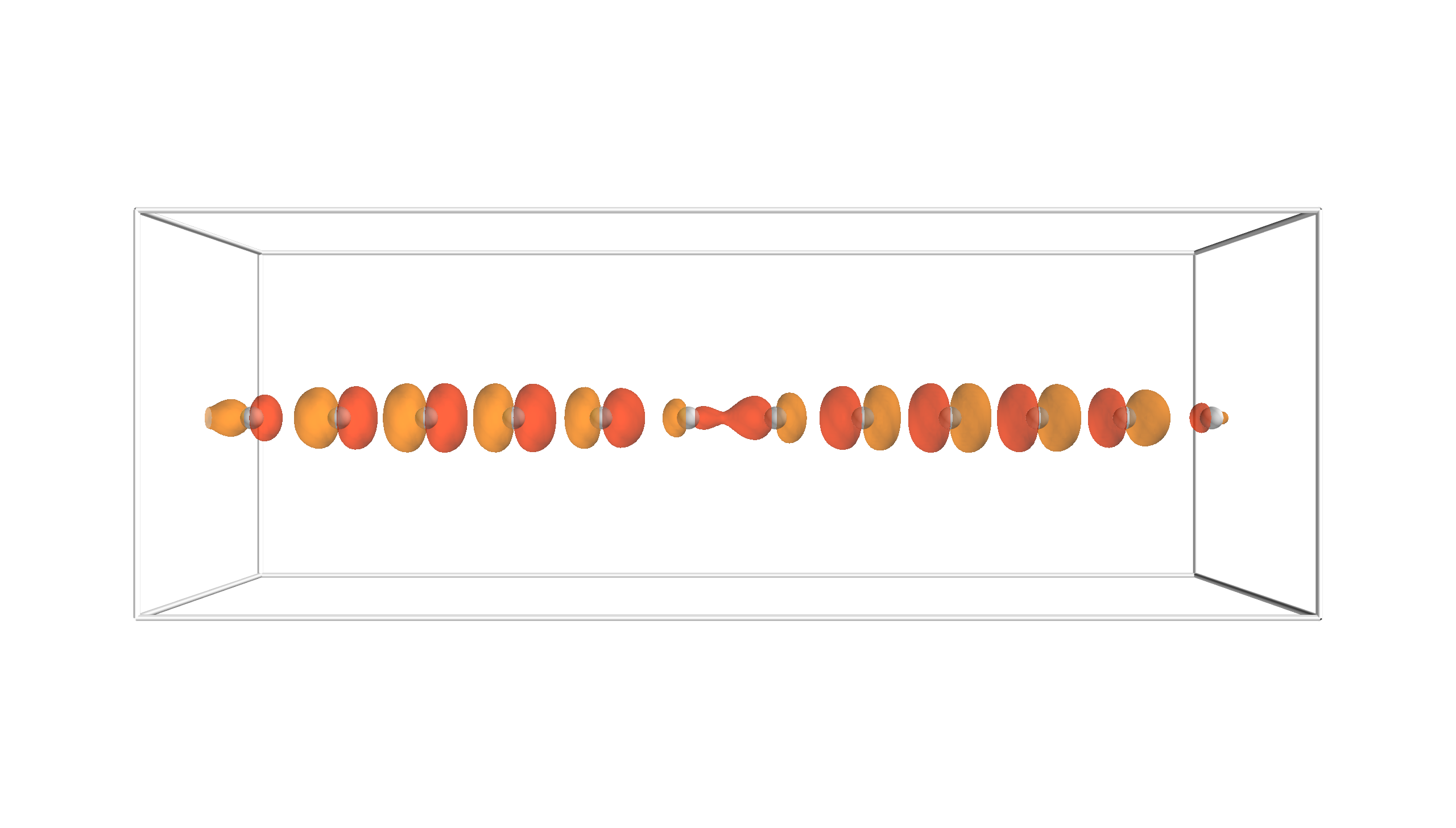
Fig. 3 Scattered wave carbon chain

[1]

Khomyakov, P. A., Brocks, G., Karpan, V., Zwierzycki, M., & Kelly, P. J. (2005). Conductance calculations for quantum wires and interfaces: Mode matching and Green’s functions. Physical Review B, 72(3), 035450.

[2]

Sørensen, H. H. B., Hansen, P. C., Petersen, D. E., Skelboe, S., & Stokbro, K. (2009). Efficient wave-function matching approach for quantum transport calculations. Physical Review B, 79(20), 205322.