Spintronics tutorial

Requirements

Software components

• nanotools

• NanoDCAL+

References

• J.Maassen, W. Ji and H. Guo, Nano. Lett., 11, 151 (2011)

Pseudopotentials

• C_LDA_TM_DZP.mat

• Ni_LDA_TM_DZP.mat

Copy the mat files from the pseudo database to the current working directory and export NANODCALPLUS_PSEUDO=$PWD.

Structure files

• c_ni_left.xyz

• c_ni_right.xyz

• c_ni_center.xyz

Briefing

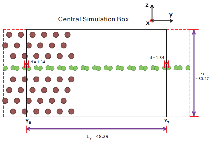
In this tutorial, we simulate the transport property of a graphene - spintronic device consisting of a single graphene sheet embedded in spin-polarized nickel. The model is sketched in the figure below. Transport occurs along the y-axis, and the structure is periodic along x,z-axes.

Script

The full python script for our calculation is as follows:

from nanotools import Atoms, Cell, System, TotalEnergy, Transmission, TwoProbe

npc = 40  # number of processors to be used

# set up TotalEnergy calculator for left lead
cell = Cell(
    avec=(
        [
            [4.64682193271677, 0.0, 0.0],
            [0.0, 8.04853168139326, 0.0],
            [0.0, 0.0, 30.27076472739540],
        ],
        "bohr",
    ),
    resolution=(0.2, "bohr"),
)
atoms = Atoms(positions=("c_ni_left.xyz", "bohr"))
sys = System(cell=cell, atoms=atoms)
sys.hamiltonian.ispin = 2
sys.atoms.set_initial_magnetic_moments("c_ni_left.xyz")
sys.kpoint.set_grid([10, 40, 1])
sys.pop.type = "fd"
left = TotalEnergy(sys)
left.solver.mix.alpha = 0.02
left.solver.mix.precond = "kerker"
left.solver.mix.maxit = 150
left.solver.mix.tol = 1.0e-6
left.solver.restart.densityPath = "left_out.h5"
left.solver.set_mpi_command(f"mpiexec -n {npc}")
left.solver.mpidist.kptprc = npc

# set up TotalEnergy calculator for right lead
cell = Cell(
    avec=(
        [
            [4.64682193271677, 0.0, 0.0],
            [0.0, 8.04853168139326, 0.0],
            [0.0, 0.0, 30.27076472739540],
        ],
        "bohr",
    ),
    resolution=(0.2, "bohr"),
)
atoms = Atoms(positions=("c_ni_right.xyz", "bohr"))
sys = System(cell=cell, atoms=atoms)
sys.hamiltonian.ispin = 2
sys.pop.type = "fd"
sys.atoms.set_initial_magnetic_moments("c_ni_right.xyz")
sys.kpoint.set_grid([10, 40, 1])
right = TotalEnergy(sys)
right.solver.mpidist.kptprc = npc
right.solver.set_mpi_command(f"mpiexec -n {npc}")

# set up TotalEnergy calculator for central region
cell = Cell(
    avec=(
        [
            [4.64682193271677, 0.0, 0.0],
            [0.0, 48.29119008835956, 0.0],
            [0.0, 0.0, 30.27076472739540],
        ],
        "bohr",
    ),
    resolution=(0.2, "bohr"),
)
atoms = Atoms(positions=("c_ni_center.xyz", "bohr"))
sys = System(cell=cell, atoms=atoms)
sys.hamiltonian.ispin = 2
sys.atoms.set_initial_magnetic_moments("c_ni_center.xyz")
sys.kpoint.set_grid([10, 1, 1])
sys.pop.type = "fd"
center = TotalEnergy(sys)

# solver parameters
center.solver.mix.alpha = 0.02
center.solver.mix.precond = "kerker"
center.solver.mix.maxit = 300
center.solver.mix.tol = 1.0e-6
center.solver.mpidist.kptprc = 10
center.solver.set_mpi_command(f"mpiexec -n {npc}")
center.solver.restart.densityPath = "center_out.h5"
# center.solver.cache_self_energy = False  #default: True

# initialize TwoProbe calculator and perform self-consistent calculation
# transport occurs along y-axis (transport_axis=1)
dev = TwoProbe(left=left, center=center, right=right, transport_axis=1)
dev.solve()

# transmission calculation
# initialized transmission calculator from that for twoprobe
trs = Transmission.from_twoprobe(twoprb=dev)

# increase k-point mesh density
trs.center.system.kpoint.set_grid([120, 1, 20])

# set mpi parameters
trs.center.solver.mpidist.kptprc = npc
trs.center.solver.set_mpi_command(f"mpiexec -n {npc}")

# compute transmission at 0.1 eV
trs.solve(energies=0.1)
trs.plot(filename="spin_trsm.png")

structure file c_ni_left.xyz, in Cartesian coordinates

18
s x y z sz
Ni   1.16170546635838   0.67334134069663   5.56546536369770   1
Ni   1.16170546635838   0.68561034069663  24.71659336369770   1
Ni   3.48511646635838   2.00966934069663   9.25741636369770   1
Ni   3.48511646635838   2.01767134069663  28.41489436369770   1
Ni   1.16170546635838   3.35594834069663  12.95920936369770   1
Ni   1.16170546635838   3.35776134069663   1.85587036369770   1
Ni   1.16170546635838   3.36359234069663  21.01628036369770   1
Ni   3.48511646635838   4.69760734069663   5.56546536369770   1
Ni   3.48511646635838   4.70987734069663  24.71659336369770   1
Ni   1.16170546635838   6.03393534069663   9.25741636369770   1
Ni   1.16170546635838   6.04193834069663  28.41489436369770   1
Ni   3.48511646635838   7.38021634069663  12.95920936369770   1
Ni   3.48511646635838   7.38203034069663   1.85587036369770   1
Ni   3.48511646635838   7.38786034069663  21.01628036369770   1
C    1.16170546635838   0.67050034069663  16.79453236369770   1
C    1.16170546635838   3.35376234069663  16.95164236369770   1
C    3.48511646635838   4.69476834069663  16.79453236369770   1
C    3.48511646635838   7.37803134069663  16.95164236369770   1

structure file c_ni_right.xyz, in Cartesian coordinates

4
s x y z sz
C     1.16170546635838  3.35586034069663   16.96215117189000 0.0
C     1.16170546635838  0.67290534069663   16.96711717189000 0.0
C     3.48511646635838  7.38012834069663   16.96215117189000 0.0
C     3.48511646635838  4.69717334069663   16.96711717189000 0.0

structure file c_ni_center.xyz, in Cartesian coordinates

52
s x y z sz
Ni   1.16170546635838   0.67334134069663   5.56546536369770   0.5
Ni   1.16170546635838   0.68561034069663  24.71659336369770   0.5
Ni   3.48511646635838   2.00966934069663   9.25741636369770   0.5
Ni   3.48511646635838   2.01767134069663  28.41489436369770   0.5
Ni   1.16170546635838   3.35594834069663  12.95920936369770   0.5
Ni   1.16170546635838   3.35776134069663   1.85587036369770   0.5
Ni   1.16170546635838   3.36359234069663  21.01628036369770   0.5
Ni   3.48511646635838   4.69760734069663   5.56546536369770   0.5
Ni   3.48511646635838   4.70987734069663  24.71659336369770   0.5
Ni   1.16170546635838   6.03393534069663   9.25741636369770   0.5
Ni   1.16170546635838   6.04193834069663  28.41489436369770   0.5
Ni   3.48511646635838   7.38021634069663  12.95920936369770   0.5
Ni   3.48511646635838   7.38203034069663   1.85587036369770   0.5
Ni   3.48511646635838   7.38786034069663  21.01628036369770   0.5
Ni   1.16170546635838   8.72187302208989   5.56546536369770   0.5
Ni   1.16170546635838   8.73414202208989  24.71659336369770   0.5
Ni   3.48511646635838  10.05820102208989   9.25741636369770   0.5
Ni   3.48511646635838  10.06620302208989  28.41489436369770   0.5
Ni   1.16170546635838  11.40448002208989  12.95920936369770   0.5
Ni   1.16170546635838  11.40629302208989   1.85587036369770   0.5
Ni   1.16170546635838  11.41212402208989  21.01628036369770   0.5
Ni   3.48511646635838  12.74613902208989   5.56546536369770   0.5
Ni   3.48511646635838  12.75840902208989  24.71659336369770   0.5
Ni   1.16170546635838  14.08246702208989   9.25741636369770   0.5
Ni   1.16170546635838  14.09047002208989  28.41489436369770   0.5
Ni   3.48511646635838  15.42874802208989  12.95920936369770   0.5
Ni   3.48511646635838  15.43056202208989   1.85587036369770   0.5
Ni   3.48511646635838  15.43639202208989  21.01628036369770   0.5
C    1.16170546635838   0.67050034069663  16.79453236369770   0.05
C    1.16170546635838   3.35376234069663  16.95164236369770   0.05
C    3.48511646635838   4.69476834069663  16.79453236369770   0.05
C    3.48511646635838   7.37803134069663  16.95164236369770   0.05
C    1.16170546635838   8.71903202208989  16.79453236369770   0.05
C    1.16170546635838  11.40229402208989  16.95164236369770   0.05
C    3.48511646635838  12.74330002208989  16.79453236369770   0.05
C    3.48511646635838  15.42656302208989  16.95164236369770   0.05
C    1.16170546635838  16.76756370348315  16.79453236369770   0.00
C    1.16170546635838  19.45082570348315  16.95164236369770   0.00
C    3.48511646635838  20.79183170348315  16.79453236369770   0.00
C    3.48511646635838  23.47509470348315  16.95164236369770   0.00
C    1.16170546635838  24.81609538487641  16.79453236369770   0.00
C    1.16170546635838  27.49935738487641  16.95164236369770   0.00
C    3.48511646635838  28.84036338487641  16.79453236369770   0.00
C    3.48511646635838  31.52362638487641  16.95164236369770   0.00
C    1.16170546635838  32.86462706626967  16.79453236369770   0.00
C    1.16170546635838  35.54788906626968  16.95164236369770   0.00
C    3.48511646635838  36.88889506626967  16.79453236369770   0.00
C    3.48511646635838  39.57215806626967  16.95164236369770   0.00
C    1.16170546635838  40.91315874766293  16.79453236369770   0.00
C    1.16170546635838  43.59642074766293  16.95164236369770   0.00
C    3.48511646635838  44.93742674766293  16.79453236369770   0.00
C    3.48511646635838  47.62068974766294  16.95164236369770   0.00

Explanations

The script starts by defining TotalEnergy calculators for the three separate regions of the transport structure. For each region we have one .xyz file to specify the atomistic structure, where initial magnetic moments at individual atomic sites are also specified in the sz column. Collinear spin polarization is turned on by

sys.hamiltonian.ispin = 2

As for solver parameters we specify using the Kerker mixing algorithm, which is generally preferable for metallic systems such as ours.

Note that in this tutorial we have enabled (by default) the program to cache lead self-energies so as to avoid computing them repetitively on the fly. However, under limited memory resource, one may want to disable this caching feature by

center.solver.cache_self_energy = False

In doing so, each iteration during the self-consistent calculation may take significantly longer time.

The self-consistent calculation typically takes many iterations to converge. If convergence is not reached after mix.maxit iterations, run the following script to restart the calculation

from nanotools import TwoProbe
dev = TwoProbe.read(filename="nano_2prb_in.json")
dev.center.solver.mix.alpha = 0.05 # play with it!
dev.center.solver.restart.densityPath = "center_out.h5"
dev.solve()

Adjusting the mix.alpha parameter may also help.

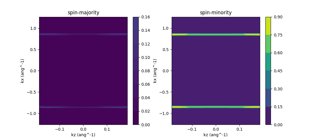
The last part of our script is dedicated to transmission calculation. The transmission of our system is supposed to be a three dimensional function along the two periodic axes plus one energy dimension. For illustrative purpose we only compute the transmission at a single energy point. The resulting plot, saved as “spin_trsm.png” in file system, should look like the following

One may also use the following script to launch a transmission calculation, separate from the self-consistent calculation:

from nanotools import TwoProbe, Transmission
dev = TwoProbe.read(filename="nano_2prb_out.json")
trs = Transmission.from_twoprobe(twoprb=dev)
trs.center.system.kpoint.set_grid([120,1,20])
trs.center.solver.mpidist.kptprc = 40
trs.center.solver.set_mpi_command("mpiexec -n 40")
trs.solve(energies=0.1, unit="ev")
trs.plot(filename="spin_trsm.png")

A quick remark on our result. We notice that the transmission is mainly focused on two lines in the whole Brillouin zone. The x coordinate of the lines actually correspond to the projected position of graphene Dirac points, where electrons can tunnel through.