3. General considerations

On this page, we discuss general considerations regarding usage of QTCAD.

3.1. Units

In QTCAD, all units are SI base units by default. This means that distances are expressed in meters, masses in kilograms, energies in Joules, etc.

To clarify units, each Theory section includes a table of relevant object attributes which specifies units that are assumed in the QTCAD API.

3.2. Elements, local nodes, and global nodes

To manipulate quantities relevant to QTCAD simulations, it is important to distinguish between elements, local nodes, and global nodes.

To better make this distinction, it is useful to start from an example. Fig. 3.2.1 illustrates a simple two-dimensional mesh.

The mesh contains several elements, labeled by the index \(e\) in the figure. In this mesh, these are first-order Lagrange elements, corresponding to triangles. Each element contains several local nodes, labeled by the index \(j\) for each element. Each local node is uniquely identified by the couple of indices \((e,j)\). In addition, it is possible to label those same nodes using a single global node index \(k\), instead.

Distinguishing between local and global nodes is particularly useful in the presence of discontinuous interfaces between materials. In such a situation, a parameter may be given a different value at two local nodes that correspond to the same global node. For example, at the interface between elements \(2\) and \(3\) in Fig. 3.2.1, local nodes \((3,0)\) and \((3,2)\) may be assigned parameter values that differ from those of \((2,0)\) and \((2,1)\), even though they correspond to the same pair of global nodes.

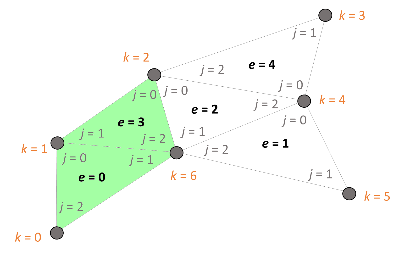
Fig. 3.2.1 Elements, local nodes, and global nodes

3.3. Parameters and variables

In the partial differential equations (PDEs) solved by QTCAD, we distinguish parameters from variables.

Parameters are the known quantities in the PDEs being solved. By contrast, variables are the unknown quantities that the differential equations are being solved for. For example, in Poisson’s equation

\[\nabla\cdot\left(\varepsilon\nabla\varphi\right)=-\rho,\]

the dielectric permittivity \(\varepsilon\) and charge density \(\rho\) are parameters, while the electric potential \(\varphi\) is the variable of interest.

This distinction may seem excessively formal. However, parameters and variables are treated differently in QTCAD in terms of data structure.

Parameters are stored either as 1D or 2D arrays. In the case of a 1D array, each entry contains the value of the parameter at an element of the mesh; this assumes that the parameter is constant over each element. For example, this is the case when a parameter is determined purely by the material type. In the case of a 2D array, each entry corresponds to the value of the parameter at a specific local node of an element. In this situation, the row index refers to the element, while the column index refers to the local node inside the element.

By contrast, variables are stored at global nodes of the mesh. This is a consequence of the fact that QTCAD uses the finite-element method, which produces a solution at each global node.

In the Theory section, parameters and variables that are relevant to each PDE are clearly distinguished.

3.3.1. Parameter setters

Typically, parameter values are automatically assigned to each element or local node when specifying materials of each region of a device. However, in some circumstances, it may be useful to manually modify parameter values. In such cases, this should be done through setters, i.e. methods of the Device class specifically designed to modify parameter values. Appropriate setters for each device parameter are tabulated in the relevant Theory sections.

When parameters are functions of space, there are four main ways to specify them. For a fictitious parameter called param, calling the corresponding setter for a device dvc will look like this:

dvc.set_param(values, region=region)

There are four main ways to set parameter values.

1. Using global nodes. In this case, region should be None (its default value), and values should be a 1D array giving the value of the parameter at each global node of the device’s mesh. For example:

   x, y, z = dvc.mesh.glob_nodes.T
   values = 0.5*x**2 + 2.5*y**2 + 3.0*z**2
   dvc.set_param(values)
   

2. Using local nodes. In this case, region should be None (its default value), and values should be a 2D array giving the value of the parameter at each local node of the device’s mesh. In the array, the row index corresponds to elements, and the column index to local nodes inside each element. For example:

   x, y, z = dvc.mesh.loc_node_coords()
   values = 0.5*x**2 + 2.5*y**2 + 3.0*z**2
   dvc.set_param(values)
   

3. Using a function of position. In this case, region should be None (its default value), and values should be a callable function of Cartesian coordinate \(x\), \(y\), and \(z\). The function should be compatible with \(x\), \(y\), and \(z\) being 1D arrays giving all global node coordinate values. For example:

   def my_func(x,y,z):
       return 0.5*x**2 + 2.5*y**2 + 3.0*z**2
   
   dvc.set_param(my_func)
   

4. Using regions. In this case, region should be the string labeling a physical region, while values should be a float giving the value of the parameter assumed constant throughout this region.

   For example:

   dvc.set_param(1.0, region="region_label")
   

Note

Methods 1 and 2 will not work for adaptive meshes since they do not allow updating device parameters when the mesh is refined. When using adaptive meshing, methods 3 and 4 should be preferred.

3.4. Finite elements

In the finite-element method, physical quantities are discretized using shape functions. Shape functions are real functions of space of the form \(\phi_j^e(\mathbf{r})\), where \(e\) and \(j\) are element and local-node indices, respectively, and \(\mathbf{r}\) is the position vector. Shape functions obey the property

\[\phi_i^e(\mathbf{r}_j^e)=\delta_{ij},\]

where \(r_j^e\) is the position of local node \((e,j)\), and \(\delta_{ij}\) is the Kronecker delta function. Functions of position are expanded over finite-element shape functions as

\[f(\mathbf{r})\approx \sum_j \phi_j^e(\mathbf r)f_j^e ,\]

where \(f_j^e\equiv f(\mathbf r_j^e)\), and it is implicitly assumed that \(\mathbf r\) lies within element \(e\).

QTCAD supports first-order and second-order Lagrange elements in dimension 1, 2, and 3. These elements correspond to lines in 1D, triangles in 2D, and tetrahedra in 3D. Shape functions for \(d\)-dimensional Lagrange elements of order \(n\) are \(d\)-dimensional polynomials of degree \(n\). The number of local nodes per element is determined by the number of unknowns in the polynomial, and thus depends on dimension and order. The following table gives the number of local nodes for each type of element supported by QTCAD.

Dimension	First order	Second order
1D	2 nodes	3 nodes
2D	3 nodes	6 nodes
3D	4 nodes	10 nodes

By default, when producing a mesh, Gmsh assumes first-order Lagrange elements.

Second-order elements and their corresponding mesh may be produced in a .geo script with

Mesh 1;
Mesh 2;
Mesh 3;
Mesh.SecondOrderLinear=1;
SetOrder 2;

Save "mesh_name.msh2";

While the command SetOrder 2 turns first-order elements into second-order elements, the command Mesh.SecondOrderLinear=1 ensures that all local nodes of the second-order elements are within the Lagrange line, triangle, or tetrahedron, which may not otherwise be the case for round boundaries.

Typically, QTCAD simulations are done with first-order meshes, which are easier to code and to use. However, second-order meshes may allow better precision for the same computational resources in some cases, in particular for the Schrödinger solver.