4. Calculating the Energy Spectrum as a Function of Detuning

4.1. Requirements

4.1.1. Software components

• QTCAD

• NumPy

• SciPy

• Matplotlib

4.1.2. Python scripts

• qtcad/examples/practical_application/Tunnel_Falls_DAPS/2-energy_vs_detuning.py

• qtcad/examples/practical_application/Tunnel_Falls_DAPS/double_dot_tunnel_falls.py

• qtcad/examples/practical_application/Tunnel_Falls_DAPS/valley_kp_model.py

4.1.3. References

• Mesh generation using QTCAD Builder

• Creating the Tunnel Falls Device

• Position-Dependent Two-Valley \mathbf{k} \cdot \mathbf{p} Model

4.2. Briefing

This final script computes the single-particle energy spectrum as a function of the detuning between the P5 and P6 plunger gates.

The energy spectrum can be useful because it shows where states localized in different dots or valleys approach one another, hybridize, and form anticrossings as the plunger-gate detuning is swept. The positions and sizes of these avoided crossings encode the orbital tunnel coupling, valley mixing, and local electrostatic lever arms of the double-dot system.

This is closely related to dipolar anticrossing spectroscopy (DAPS). In DAPS, the measured response is sensitive to changes in the electric dipole moment of the electron states of the double-dot system as a function of detuning. These changes are strongest near anticrossings where the electron charge distribution changes rapidly from being localized in one dot to being localized in the other. The spectrum computed here therefore identifies the detuning regions where the DAPS signal is expected to be strongest.

4.3. Setup

4.3.1. Header

We start by importing the relevant modules. This script imports QTCAD’s linear Poisson Solver and Schrödinger Solver, the Device generation helper get_double_dot_tunnel_falls defined in double_dot_tunnel_falls.py, the save_slice and state_probability_density helpers used for diagnostic wavefunction-density plots, and the position-dependent two-valley \(\mathbf{k} \cdot \mathbf{p}\) model helper generate_correlated_two_valley_model defined in valley_kp_model.py.

from pathlib import Path
import matplotlib.pyplot as plt
import numpy as np
from qtcad.device import Device, SubDevice
from qtcad.device import constants as ct
from qtcad.device.mesh3d import SubMesh
from qtcad.device.poisson_linear import Solver as LinearPoissonSolver
from qtcad.device.poisson_linear import SolverParams as LinearPoissonSolverParams
from qtcad.device.schrodinger import Solver as SchrodingerSolver
from qtcad.device.schrodinger import SolverParams as SchrodingerSolverParams
from double_dot_tunnel_falls import (
    get_double_dot_tunnel_falls,
    save_slice,
    state_probability_density,
)
from double_dot_tunnel_falls import V_B4, V_P5, V_B5, V_B6, V_SG, V_CS
from valley_kp_model import generate_correlated_two_valley_model

4.3.2. File paths

Next, we define the paths to the solver input files and to the output files for the calculation results:

# File paths.
script_dir = Path(__file__).parent.resolve()
mesh_dir = script_dir / "meshes"
path_out = script_dir / "output"
path_local_out = path_out / "energy_vs_detuning"
path_local_out.mkdir(parents=True, exist_ok=True)

mesh_file = mesh_dir / "tunnel_falls_double_dot.msh"
geo_file = mesh_dir / "tunnel_falls_double_dot.xao"
refined_mesh_file = mesh_dir / "refined_tunnel_falls_double_dot.msh"

valley_map_file = path_local_out / "valley_splitting_map.png"
energy_spectrum_file = path_local_out / "energy_spectrum.txt"
energy_spectrum_plot_file = path_local_out / "energy_spectrum.png"
ground_state_density_files = [
    path_local_out / "ground_state_density_negative_detuning.png",
    path_local_out / "ground_state_density_positive_detuning.png",
]

The variables mesh_file and geo_file contain the paths to the coarse mesh and geometry file generated by Mesh generation using QTCAD Builder.

4.3.3. Simulation parameters

We now define the simulation parameters. This includes an array detuning_values which defines the plunger-gate detuning sweep. The plunger detuning is swept symmetrically around the common center plunger voltage.

# Detuning sweep.
V_P_center = V_P5
Delta_V = 0.01
num_voltages = 11
detuning_values = np.linspace(-Delta_V, Delta_V, num_voltages)

We also set the parameters of the position-dependent two-valley \(\mathbf{k} \cdot \mathbf{p}\) model. These parameters define the spatial valley-coupling map used in the Schrödinger equation. The mean value sets the average valley splitting over the device, while the correlation lengths control how quickly the valley coupling varies in the \(x\) and \(y\) directions. The parameters map_nx and map_ny set the number of sampling points used to generate this map, and random_seed fixes the particular disorder realization so that the calculation is reproducible.

# Correlated valley-splitting parameters.
mean_valley_splitting = 200.0e-6 * ct.e
correlation_length_x = 19.2e-9
correlation_length_y = 1000e-9
map_nx = 200
map_ny = 15
random_seed = 8

Here, mean_valley_splitting, the mean valley splitting, is set to 200 \(\mu\mathrm{eV}\), and correlation_length_x, the valley-splitting correlation length along \(x\), is set to 19.2 \(\mathrm{nm}\). Both parameters are taken from experimental values for the Tunnel Falls device [MEB+25]. In that work, only correlations along the \(x\) direction were considered. We therefore set the correlation length along \(y\), correlation_length_y, to a much larger value, making the valley-splitting map nearly constant in the \(y\) direction. To include appreciable variations along \(y\), correlation_length_y can be decreased to a value comparable to the length scale over which such variations are expected to occur.

4.3.4. Gate voltages

For convenience, we also create a function that produces a dictionary of gate voltages for a given value of detuning. This function will be useful for solving the Poisson equation for different voltage configurations.

def gate_biases_for_detuning(detuning: float) -> dict[str, float]:
    """Return the gate voltages used for one detuning point.

    Args:
        detuning: Symmetric P5-P6 detuning in volts. Positive detuning raises
            ``P5`` and lowers ``P6`` by the same amount.

    Returns:
        Dictionary of gate voltages accepted by the linear Poisson solver.
    """
    return {
        "V_B4": V_B4,
        "V_P5": V_P_center + 0.5 * detuning,
        "V_B5": V_B5,
        "V_P6": V_P_center - 0.5 * detuning,
        "V_B6": V_B6,
        "V_SG": V_SG,
        "V_CS": V_CS,
    }

4.4. Solving the linear Poisson equation

Next, we create a function that solves the linear Poisson equation for a given set of gate voltages. The function takes a dictionary of gate biases, a mesh file, an optional geometry file and an output path for a refined mesh.

The function first creates a Device using the get_double_dot_tunnel_falls function. It then configures and solves the linear Poisson equation. After the electrostatic potential has been computed, the function sets the confinement potential on the Device using set_V_from_phi. Finally, it returns the same Device, together with the region labels identifying the left and right quantum dots.

The Device created by solve_linear_poisson is defined on the input Mesh with filename mesh_file_name. If geo_file_name is not None, adaptive meshing is enabled. In that case, the Solver generates a refined mesh and, if refined_mesh_file is provided, saves it to that path.

def solve_linear_poisson(
    gate_biases: dict[str, float],
    *,
    mesh_file_name: str | Path = mesh_file,
    geo_file_name: str | Path | None = None,
    refined_mesh_file: str | Path | None = None,
) -> tuple[Device, list[str], list[str]]:
    """Solve the linear Poisson equation for one gate configuration.

    Args:
        gate_biases: Dictionary of gate voltages accepted by the Poisson solve.
        mesh_file_name: Mesh file used to create the device.
        geo_file_name: Geometry file used to activate adaptive meshing. When
            omitted, the Poisson equation is solved on the input mesh without
            adaptive meshing.
        refined_mesh_file: Output path for the refined mesh written by the
            adaptive solve.

    Returns:
        Device with solved potential, left-dot region labels, and right-dot
        region labels.
    """

    # Create the device.
    device, left_dot_region, right_dot_region = get_double_dot_tunnel_falls(
        mesh_file_name=str(mesh_file_name),
        **gate_biases,
    )

    # Set up linear Poisson solver.
    solver_params = LinearPoissonSolverParams()
    solver_params.tol = 1e-12
    # Adaptive meshing if a geometry file is passed.
    if geo_file_name is not None:
        solver_params.eta0 = 0.30
        solver_params.refined_region = left_dot_region + right_dot_region
        solver_params.h_refined = 1.0
        if refined_mesh_file is not None:
            solver_params.refined_mesh_filename = str(refined_mesh_file)
    solver = LinearPoissonSolver(
        d=device,
        solver_params=solver_params,
        geo_file=geo_file_name,
    )

    solver.solve()
    device.set_V_from_phi()

    return device, left_dot_region, right_dot_region

4.5. Solving the Schrödinger equation

The helper below configures and runs the single-particle Schrödinger Solver on a Device.

def solve_schrodinger(
    subdevice: Device | SubDevice,
    *,
    num_states: int = 8,
    tol: float = 1e-12,
) -> Device | SubDevice:
    """Solve the single-particle Schrödinger equation on a dot subdevice.

    Args:
        subdevice: Dot subdevice on which the solve is performed.
        num_states: Number of eigenstates requested from the solver.
        tol: Schrödinger solver tolerance.

    Returns:
        The solved subdevice.
    """
    # Schrödinger solver parameters.
    solver_params = SchrodingerSolverParams()
    solver_params.num_states = num_states
    solver_params.tol = tol

    # Force wavefunctions to 0 at the edges.
    subdevice.set_insulator_boundaries()

    solver = SchrodingerSolver(subdevice, solver_params=solver_params)
    solver.solve()
    return subdevice

Before solving the Schrödinger equation, we impose hard-wall boundary conditions using the set_insulator_boundaries method. These boundary conditions force all wavefunctions to vanish at the edges of the simulation domain. This confines the eigenstates to the physical device region and suppresses spurious solutions that can otherwise arise from boundary effects.

Note

The set_insulator_boundaries method should be used with care. If the simulation domain is too small, forcing the wavefunctions to vanish at the boundary can introduce artificial confinement and shift the computed energy levels. The simulation domain should therefore be chosen large enough that the relevant wavefunctions decay well before reaching the boundary.

4.6. Energy-spectrum plot

The following helper saves a plot of the lowest energy levels as a function of detuning. Specifically, we plot the first four energy levels. In the small-detuning limit, these levels correspond to the valley-split ground orbital states in the two dots. For visualization purposes, the energy levels are plotted relative to the minimum ground-state energy obtained over the detuning sweep, \(\min E_0\).

def save_energy_spectrum_plot(
    detuning: np.ndarray,
    energy_data: np.ndarray
) -> None:
    """Save the energy spectrum as a function of detuning.

    Args:
        detuning: Detuning values.
        energy_data: Double-dot eigenenergies for different voltage detuning values.
            Each row corresponds to an entry in detuning.
    """
    energies_mev = energy_data[:, :4] * 1e3
    energies_mev -= np.nanmin(energies_mev[:, 0])

    figure, axis = plt.subplots(figsize=(6.0, 4.5))
    for state in range(energies_mev.shape[1]):
        axis.plot(
            detuning * 1000,
            energies_mev[:, state],
            marker="o",
            linewidth=1.5,
            label=f"State {state}",
        )

    axis.set_xlabel("Detuning [mV]")
    axis.set_ylabel("$E - \\min (E_0)$ [meV]")
    axis.grid(alpha=0.25)
    axis.legend(fontsize=8, ncol=2)
    figure.tight_layout()
    figure.savefig(energy_spectrum_plot_file, dpi=200)
    plt.close(figure)

4.7. Energy spectrum vs. detuning

4.7.1. Refined mesh

We now generate the final calculation. We start by running the linear Poisson Solver with adaptive meshing enabled to generate a refined Mesh written to the path specified by refined_mesh_file.

if __name__ == "__main__":

    # Generate the refined mesh.
    device, left_dot_region, right_dot_region = solve_linear_poisson(
        gate_biases_for_detuning(0.0),
        mesh_file_name=mesh_file,
        geo_file_name=geo_file,
        refined_mesh_file=refined_mesh_file,
    )

4.7.2. Valley model

Next, the dot SubMesh is extracted from the refined mesh, and the correlated two-valley \(\mathbf{k} \cdot \mathbf{p}\) model is generated on that SubMesh using the generate_correlated_two_valley_model function.

# Get k·p model on the refined mesh.
dot_region = left_dot_region + right_dot_region
dot_mesh = SubMesh(device.mesh, dot_region)

model = generate_correlated_two_valley_model(
    dot_mesh.glob_nodes[:, :2],
    mean_valley_splitting=mean_valley_splitting,
    correlation_length_x=correlation_length_x,
    correlation_length_y=correlation_length_y,
    map_nx=map_nx,
    map_ny=map_ny,
    random_seed=random_seed,
    valley_map_filename=valley_map_file
)

The generated valley-splitting map is shown in Fig. 4.7.5. As expected, there is no noticeable variation in the valley splitting along the \(y\) axis.

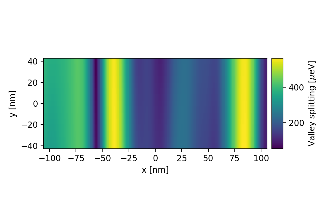
Fig. 4.7.5 Correlated valley-splitting map sampled over the double-dot region. The large correlation length along \(y\) makes the map vary primarily along the transport direction.

4.7.3. Detuning loop

Finally, we loop over the detuning values and solve the linear Poisson equation. Here, we do not pass a geo_file to the solve_linear_poisson function. We use the previously generated refined mesh, stored in the attribute mesh of device for this and all subsequent calculations. From there, we generate a SubDevice representing the quantum-dot regions. Then, we attach the ElectronKPModel generated above, before solving the Schrödinger equation.

energy_data = []

for detuning_index, detuning in enumerate(detuning_values):
    gate_biases = gate_biases_for_detuning(detuning)

    print("\n" + "=" * 60)
    print(f"Detuning point {detuning_index + 1}/{detuning_values.size}")
    print(f"detuning = {detuning:.6f} V")
    print("=" * 60)

    # Solve the linear Poisson equation.
    device, _, _ = solve_linear_poisson(
        gate_biases,
        mesh_file_name=refined_mesh_file,
    )

    # Solve the Schrödinger equation.
    dot_device = SubDevice(device, dot_mesh)
    dot_device.set_electron_kp_model(model)
    solve_schrodinger(dot_device)
    dot_device.print_energies()

    # Save ground-state density slices at the detuning-sweep endpoints.
    if detuning_index in (0, detuning_values.size - 1):
        file_index = 0 if detuning_index == 0 else 1
        save_slice(
            dot_device,
            state_probability_density(dot_device, 0),
            ground_state_density_files[file_index],
            label=r"$|\psi_0|^2$ [1 / m$^3$]",
        )

The script also saves slices of the scalar ground-state probability density at the two endpoints of the detuning sweep. These densities are computed by the state_probability_density function. At one endpoint, the electrostatic potential favors localization under one plunger gate; at the opposite endpoint, the sign of the detuning is reversed and the ground-state density shifts toward the other dot. These endpoint slices therefore illustrate how the charge configuration, and hence the electric dipole moment, changes across the detuning sweep. Tracking this charge redistribution near anticrossings is the basic idea behind dipolar anticrossing spectroscopy (DAPS) [MEB+25].

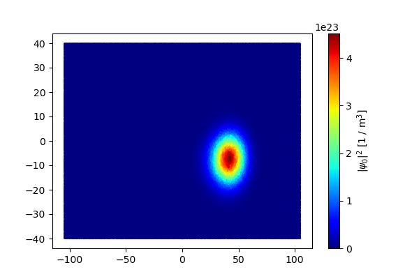
Fig. 4.7.6 Ground-state probability-density slice at the negative detuning endpoint.

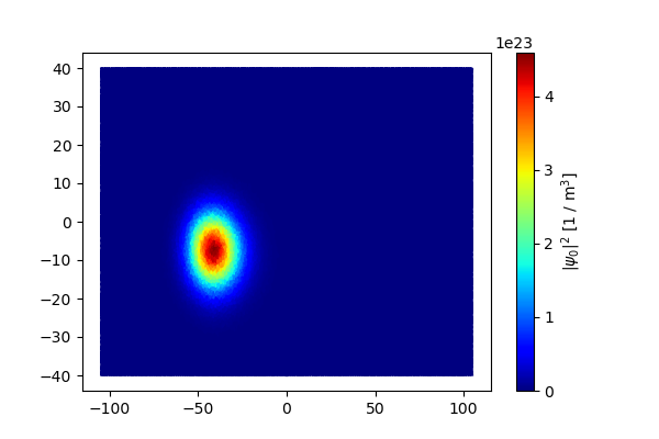
Fig. 4.7.7 Ground-state probability-density slice at the positive detuning endpoint.

Finally, the energies are saved to a file and plotted after the loop completes.

    # Save energies.
    header = "Detuning [V]    Energies [eV]"
    with open(energy_spectrum_file, "a") as f:
        out = [detuning] + list(dot_device.energies / ct.e)
        np.savetxt(f, np.array(out)[np.newaxis, :], fmt="%.8f", header=header)

    energy_data.append(dot_device.energies / ct.e)

# Plot spectrum.
energy_data = np.asarray(energy_data)
save_energy_spectrum_plot(detuning_values, energy_data)

The resulting energy spectrum is shown in Fig. 4.7.8.

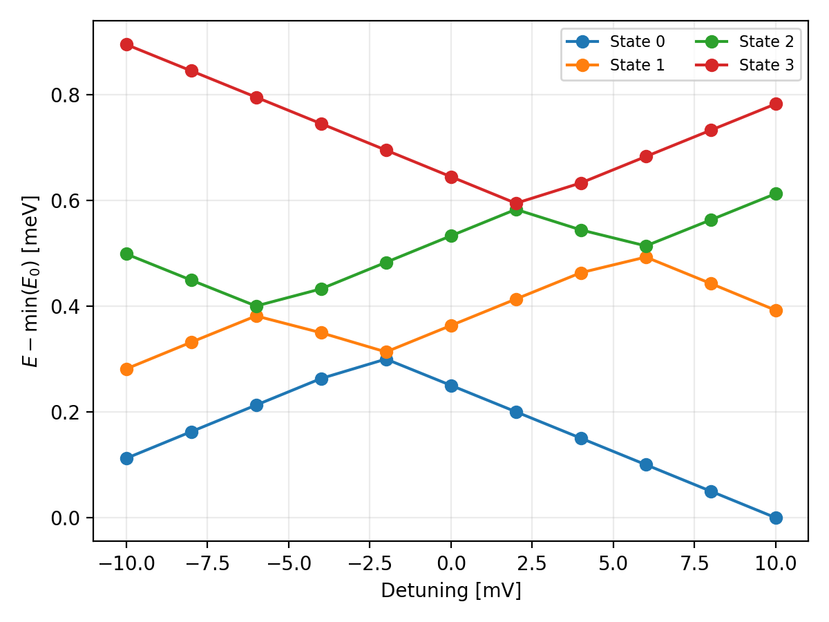
Fig. 4.7.8 Lowest single-particle energy levels as a function of the symmetric P5–P6 plunger-gate detuning. The energies are shifted by the minimum ground-state energy.

At the negative-detuning end of the plot, the ground and first excited states correspond to the valley-split states localized in the right dot, while the second and third excited states correspond to the valley-split states localized in the left dot. The spectrum shows that the valley splitting is larger in the left dot than in the right dot. As the detuning is swept, these dot-localized levels move relative to one another and undergo avoided crossings when the charge character hybridizes between the dots. Large changes in polarization are expected near these avoided crossings, which is the signal measured in DAPS.

4.8. Full code

__copyright__ = "Copyright 2022-2026, Nanoacademic Technologies Inc."

from pathlib import Path
import matplotlib.pyplot as plt
import numpy as np
from qtcad.device import Device, SubDevice
from qtcad.device import constants as ct
from qtcad.device.mesh3d import SubMesh
from qtcad.device.poisson_linear import Solver as LinearPoissonSolver
from qtcad.device.poisson_linear import SolverParams as LinearPoissonSolverParams
from qtcad.device.schrodinger import Solver as SchrodingerSolver
from qtcad.device.schrodinger import SolverParams as SchrodingerSolverParams
from double_dot_tunnel_falls import (
    get_double_dot_tunnel_falls,
    save_slice,
    state_probability_density,
)
from double_dot_tunnel_falls import V_B4, V_P5, V_B5, V_B6, V_SG, V_CS
from valley_kp_model import generate_correlated_two_valley_model

# File paths.
script_dir = Path(__file__).parent.resolve()
mesh_dir = script_dir / "meshes"
path_out = script_dir / "output"
path_local_out = path_out / "energy_vs_detuning"
path_local_out.mkdir(parents=True, exist_ok=True)

mesh_file = mesh_dir / "tunnel_falls_double_dot.msh"
geo_file = mesh_dir / "tunnel_falls_double_dot.xao"
refined_mesh_file = mesh_dir / "refined_tunnel_falls_double_dot.msh"

valley_map_file = path_local_out / "valley_splitting_map.png"
energy_spectrum_file = path_local_out / "energy_spectrum.txt"
energy_spectrum_plot_file = path_local_out / "energy_spectrum.png"
ground_state_density_files = [
    path_local_out / "ground_state_density_negative_detuning.png",
    path_local_out / "ground_state_density_positive_detuning.png",
]

# Detuning sweep.
V_P_center = V_P5
Delta_V = 0.01
num_voltages = 11
detuning_values = np.linspace(-Delta_V, Delta_V, num_voltages)

# Correlated valley-splitting parameters.
mean_valley_splitting = 200.0e-6 * ct.e
correlation_length_x = 19.2e-9
correlation_length_y = 1000e-9
map_nx = 200
map_ny = 15
random_seed = 8

def gate_biases_for_detuning(detuning: float) -> dict[str, float]:
    """Return the gate voltages used for one detuning point.

    Args:
        detuning: Symmetric P5-P6 detuning in volts. Positive detuning raises
            ``P5`` and lowers ``P6`` by the same amount.

    Returns:
        Dictionary of gate voltages accepted by the linear Poisson solver.
    """
    return {
        "V_B4": V_B4,
        "V_P5": V_P_center + 0.5 * detuning,
        "V_B5": V_B5,
        "V_P6": V_P_center - 0.5 * detuning,
        "V_B6": V_B6,
        "V_SG": V_SG,
        "V_CS": V_CS,
    }

def solve_linear_poisson(
    gate_biases: dict[str, float],
    *,
    mesh_file_name: str | Path = mesh_file,
    geo_file_name: str | Path | None = None,
    refined_mesh_file: str | Path | None = None,
) -> tuple[Device, list[str], list[str]]:
    """Solve the linear Poisson equation for one gate configuration.

    Args:
        gate_biases: Dictionary of gate voltages accepted by the Poisson solve.
        mesh_file_name: Mesh file used to create the device.
        geo_file_name: Geometry file used to activate adaptive meshing. When
            omitted, the Poisson equation is solved on the input mesh without
            adaptive meshing.
        refined_mesh_file: Output path for the refined mesh written by the
            adaptive solve.

    Returns:
        Device with solved potential, left-dot region labels, and right-dot
        region labels.
    """

    # Create the device.
    device, left_dot_region, right_dot_region = get_double_dot_tunnel_falls(
        mesh_file_name=str(mesh_file_name),
        **gate_biases,
    )

    # Set up linear Poisson solver.
    solver_params = LinearPoissonSolverParams()
    solver_params.tol = 1e-12
    # Adaptive meshing if a geometry file is passed.
    if geo_file_name is not None:
        solver_params.eta0 = 0.30
        solver_params.refined_region = left_dot_region + right_dot_region
        solver_params.h_refined = 1.0
        if refined_mesh_file is not None:
            solver_params.refined_mesh_filename = str(refined_mesh_file)
    solver = LinearPoissonSolver(
        d=device,
        solver_params=solver_params,
        geo_file=geo_file_name,
    )

    solver.solve()
    device.set_V_from_phi()

    return device, left_dot_region, right_dot_region

def solve_schrodinger(
    subdevice: Device | SubDevice,
    *,
    num_states: int = 8,
    tol: float = 1e-12,
) -> Device | SubDevice:
    """Solve the single-particle Schrödinger equation on a dot subdevice.

    Args:
        subdevice: Dot subdevice on which the solve is performed.
        num_states: Number of eigenstates requested from the solver.
        tol: Schrödinger solver tolerance.

    Returns:
        The solved subdevice.
    """
    # Schrödinger solver parameters.
    solver_params = SchrodingerSolverParams()
    solver_params.num_states = num_states
    solver_params.tol = tol

    # Force wavefunctions to 0 at the edges.
    subdevice.set_insulator_boundaries()

    solver = SchrodingerSolver(subdevice, solver_params=solver_params)
    solver.solve()
    return subdevice

def save_energy_spectrum_plot(
    detuning: np.ndarray,
    energy_data: np.ndarray
) -> None:
    """Save the energy spectrum as a function of detuning.

    Args:
        detuning: Detuning values.
        energy_data: Double-dot eigenenergies for different voltage detuning values.
            Each row corresponds to an entry in detuning.
    """
    energies_mev = energy_data[:, :4] * 1e3
    energies_mev -= np.nanmin(energies_mev[:, 0])

    figure, axis = plt.subplots(figsize=(6.0, 4.5))
    for state in range(energies_mev.shape[1]):
        axis.plot(
            detuning * 1000,
            energies_mev[:, state],
            marker="o",
            linewidth=1.5,
            label=f"State {state}",
        )

    axis.set_xlabel("Detuning [mV]")
    axis.set_ylabel("$E - \\min (E_0)$ [meV]")
    axis.grid(alpha=0.25)
    axis.legend(fontsize=8, ncol=2)
    figure.tight_layout()
    figure.savefig(energy_spectrum_plot_file, dpi=200)
    plt.close(figure)

if __name__ == "__main__":

    # Generate the refined mesh.
    device, left_dot_region, right_dot_region = solve_linear_poisson(
        gate_biases_for_detuning(0.0),
        mesh_file_name=mesh_file,
        geo_file_name=geo_file,
        refined_mesh_file=refined_mesh_file,
    )

    # Get k·p model on the refined mesh.
    dot_region = left_dot_region + right_dot_region
    dot_mesh = SubMesh(device.mesh, dot_region)

    model = generate_correlated_two_valley_model(
        dot_mesh.glob_nodes[:, :2],
        mean_valley_splitting=mean_valley_splitting,
        correlation_length_x=correlation_length_x,
        correlation_length_y=correlation_length_y,
        map_nx=map_nx,
        map_ny=map_ny,
        random_seed=random_seed,
        valley_map_filename=valley_map_file
    )

    energy_data = []

    for detuning_index, detuning in enumerate(detuning_values):
        gate_biases = gate_biases_for_detuning(detuning)

        print("\n" + "=" * 60)
        print(f"Detuning point {detuning_index + 1}/{detuning_values.size}")
        print(f"detuning = {detuning:.6f} V")
        print("=" * 60)

        # Solve the linear Poisson equation.
        device, _, _ = solve_linear_poisson(
            gate_biases,
            mesh_file_name=refined_mesh_file,
        )

        # Solve the Schrödinger equation.
        dot_device = SubDevice(device, dot_mesh)
        dot_device.set_electron_kp_model(model)
        solve_schrodinger(dot_device)
        dot_device.print_energies()

        # Save ground-state density slices at the detuning-sweep endpoints.
        if detuning_index in (0, detuning_values.size - 1):
            file_index = 0 if detuning_index == 0 else 1
            save_slice(
                dot_device,
                state_probability_density(dot_device, 0),
                ground_state_density_files[file_index],
                label=r"$|\psi_0|^2$ [1 / m$^3$]",
            )

        # Save energies.
        header = "Detuning [V]    Energies [eV]"
        with open(energy_spectrum_file, "a") as f:
            out = [detuning] + list(dot_device.energies / ct.e)
            np.savetxt(f, np.array(out)[np.newaxis, :], fmt="%.8f", header=header)

        energy_data.append(dot_device.energies / ct.e)

    # Plot spectrum.
    energy_data = np.asarray(energy_data)
    save_energy_spectrum_plot(detuning_values, energy_data)