2. Electric dipole spin resonance—Noise

2.1. Requirements

2.1.1. Software components

2.1.1.1. Basic Python modules

• numpy

• matplotlib

2.1.1.2. Specific modules

• qubit.dynamics

• qubit.noise

• qutip

2.1.2. Python script

• qtcad/examples/tutorials/EDSR_noise.py>

2.1.3. References

• Electric dipole spin resonance—Dynamics

2.2. Briefing

In this tutorial we will demonstrate how QTCAD can be used to simulate the effects of charge noise on the dynamics of a qubit. We consider the system simulated in Electric dipole spin resonance—Dynamics as a starting point and expand upon the example to include the effects of charge noise in the simulation. Specifically we will analyze the two-(lowest-energy-)level subsystem generated in Electric dipole spin resonance—Dynamics. It is assumed that the user is familiar with basic Python and has some basic familiarity with the QuTiP python library.

The full code may be found at the bottom of this page, or in EDSR_noise.py.

2.3. Header

First, a header is written to import relevant modules.

import numpy as np
from matplotlib import pyplot as plt
from device import constants as ct

import qutip
from qubit import spectra, dynamics, noise

Compared with previous tutorials, this tutorial introduces two new modules:

• spectra: Definitions of typical noise spectra (spectral density functions).

• noise: Contains tools that can be useful in simulating the effects of noise.

2.4. Problem setup

Now that the relevant modules have been imported, we set up the problem. The starting point are the system and drive Hamiltonians for the projected 2 level system analyzed in the MOS_EDSR.py example. These two operators are stored in the h0 and u variables on line 145 of the MOS_EDSR.py example. We have copied the contents of these variables here; in addition, we convert them into angular frequency units through division by \(\hbar\):

# Copied here are the Hamiltonian and drive for the projected 2 level system
# analyzed in the example `MOS_EDSR.py`. The Hamiltonian and drive are stored in the
# variables h0 and u on line 145 of `MOS_EDSR.py`.
# System Hamiltonian
h0 = np.array([[1.1128812e-23, 0.00000000e+00],
 [0.00000000e+00, 0.00000000e+00]])
H0 = h0/ct.hbar # Rewrite in units of hbar = 1
# Drive
u = np.array([[-2.03067270e-29, 1.00561612e-27-1.10285789e-37j],
 [1.00561612e-27+1.10285789e-37j, 0.+0.j]])
delta_V = u/ct.hbar # Rewrite in units of hbar = 1

We have also divided the Hamiltonians by \(\hbar\); we will be working with units where \(\hbar=1\). We note that we have chosen a system where the excited qubit state represents the first element of our basis and the ground qubit state represents the second. It is also possible to pick the opposite convention, in which case the qubit frequency will be negative (see the next block of code). In the remainder of this tutorial, we take H0 to be the system Hamiltonian for a qubit, and delta_V to be the amplitude of a drive Hamiltonian produced by a voltage applied to some gate. Thus, in what follows, we will analyze the dynamics of a qubit subject to the Hamiltonian \(H\left(t\right)=H_0 + \delta V f\left(t\right)\), where \(f\left(t\right)\) is, as of yet, an unspecified function of time.

Next, we define the relevant frequencies/time scales of the problem.

omega = np.absolute(H0[0,0] - H0[1,1]) # qubit frequency
omega_Rabi = np.absolute(delta_V[0,1]) # Rabi frequency on resonance
T_Rabi = 2*np.pi/omega_Rabi # Rabi period

The variable omega contains the qubit frequency. Given the convention chosen above (excited state energy in the top left corner of H0), omega is positive. If the opposite convention were chosen (excited state energy in the bottom right corner of H0), omega would be negative. We have neglected the contribution to the qubit frequency from delta_V, because this contribution is negligible compared to the contribution from H0 (delta_V[0, 0] is roughly 6 orders of magnitude smaller than omega). The variable omega_Rabi contains the qubit Rabi frequency on resonance and T_Rabi contains the Rabi period which will be used to define the time scales of the problem. We define the total simulation time to be T (20 Rabi periods), and will simulate the dynamics at 1000 equally spaced points from 0 to T.

T = 20 * T_Rabi # Total time of the simulations
times = np.linspace(0, T, 1000) # Times at which dynamics are simulated.

Finally, in the last stage of the setup procedure, we initialize Dynamics() and Noise() objects that will provide tools to simplify the dynamics simulations and to include noise in the problem, respectively.

# Initialize objects that will handle dynamics and noise.
dyn = dynamics.Dynamics()
N = noise.Noise()

2.5. Simple simulation - No noise

The first simulation we perform in this tutorial is a simple example in which we take \(f\left(t\right)=\cos\left(\omega t\right)\) (where \(\omega =\) omega, the qubit frequency). Thus, we simulate the dynamics for a qubit under the influence of the Hamiltonian \(H\left(t\right)=H_0+ \delta V \cos\left(\omega t\right)\). This is the same example solved in Electric dipole spin resonance—Dynamics. Here, with the help of the dyn, the Dynamics() object, we solve this problem in a rotating frame. The H_RF method—which takes as input the system Hamiltonian, H0, the drive Hamiltonian, delta_V, and frequency, omega—outputs the time-dependent Hamiltonian \(H\left(t\right)\), in a frame rotating with frequency omega around the \(z\) axis of the qubit. We also choose an initial state psi0 and run the simulation using the qutip.mesolve method.

# The Hamiltonian H = H0 + delta_V cos(omega*t) in a frame rotating
# at frequency omega.
H = dyn.H_RF(H0, delta_V, omega)
# Solve for the dynamics without any noise.
psi0 = qutip.basis(2, 0) # initial state
result0 = qutip.mesolve(H, psi0, times)

We then plot \(\braket{\sigma_z \left(t\right)}\) and \(\braket{\sigma_y \left(t\right)}\). We use qutip.expect() to calculate the expectation values at different times.

# Plot expectation values of sigma_z and sigma_y as a function of time.
fig, axes = plt.subplots(2)
fig.set_size_inches((8,8))
#<sigma_z (t)>
axes[0].plot(result0.times, qutip.expect(qutip.sigmaz(), result0.states))
#<sigma_y (t)>
axes[1].plot(result0.times, qutip.expect(qutip.sigmay(), result0.states))
# Labels
axes[0].set_ylabel(f'$\left< \sigma_z (t) \\right>$', fontsize=20)
axes[1].set_ylabel(f'$\left< \sigma_y (t) \\right>$', fontsize=20)
axes[0].set_xlabel(f'$t \, (s)$', fontsize=20)
axes[1].set_xlabel(f'$t \, (s)$', fontsize=20)
plt.show()

The plots produced are as follows.

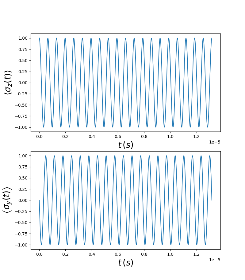
Fig. 2.5.4 Expectation values of \(\sigma_z\) and \(\sigma_y\) as a function of time.

As expected, the plots contain 20 Rabi cycles and the two plots are out of phase by an angle \(\frac{\pi}{2}\).

2.6. Generating noise

Now that we have gone through a simple example, we will generate some noise from a given spectrum and simulate how this noise affects the results presented above. The goal is therefore to generate a Hamiltonian \(H\left(t\right)=H_0 + \delta V\left[1+\beta\left(t\right)\right]\cos\left(\omega t\right)\), where \(\beta\left(t\right)\) is a stationary and ergodic Gaussian random process with vanishing mean. It represents some charge noise acting on the gate which is driving the qubit. More theoretical background on noisy EDSR is given in the subsection called A more realistic scenario: noisy electric-dipole spin resonance in the Quantum control theory section.

To generate \(\beta\left(t\right)\), we first define a spectrum for the noise. Here we select a Lorentzian spectrum centered at \(\omega=0\) with width equal to the Rabi frequency, omega_Rabi. Because the process is generated as a Fourier series, we also define a time scale T0 which must be much longer than any other time scale in the problem (\(T_0 > 20 T_{\textrm{Rabi}}\)). This time scale T0 artificially enforces some periodicity on the noisy time series generated; however, this periodicity should happen only over a very long time compared with the simulation time to correctly approximate the noise process. T0 also determines the resolution of the spectrum. Here we take T0 = 50 * T_Rabi, however this can be increased to obtain higher quality results. For purposes of this tutorial, the value chosen for T0 is sufficiently large. Thus, we generate an array of Fourrier harmonics of the process \(\beta\left(t\right)\) which are stored in wk and evaluate the Lorentzian spectrum at each of these harmonics using the spectra.lorentz function.

# Include charge noise which is assumed to affect only the gate which
# generates the drive delta_V.
# Lorentzian spectrum
S0 = 0.01 # Total power
wc = omega_Rabi # Cutoff frequency
w0 = 0 # Central frequency
# T0 should be much larger than the largest time scale of the problem under consideration.
# Used to properly define the Fourier series of the time series related to the noise.
T0 = 50 * T_Rabi  # Must take T0 such that 2*pi/T0 << wc to resolve the spectrum
omega_max = 5*wc
wk = np.arange(0, omega_max , 2*np.pi/T0) + w0
spectrum = spectra.lorentz(wk, S0, wc, w0 = w0)

We note that this approach assumes the spectrum to be symmetric around \(\omega =0\), i.e. the noise process is a classical stochastic process. Here we plot the spectrum only for values of \(\omega >0\).

# Plot spectrum
fig, axes = plt.subplots(1)
fig.set_size_inches((10,6))
axes.plot(wk, spectrum)
axes.set_ylabel(f'$S_\\beta(\omega) \, (s)$', fontsize=20)
axes.set_xlabel('$\omega \, (s^{-1})$', fontsize=20)
axes.set_title('Lorentzian spectral density', fontsize=30)
plt.show()

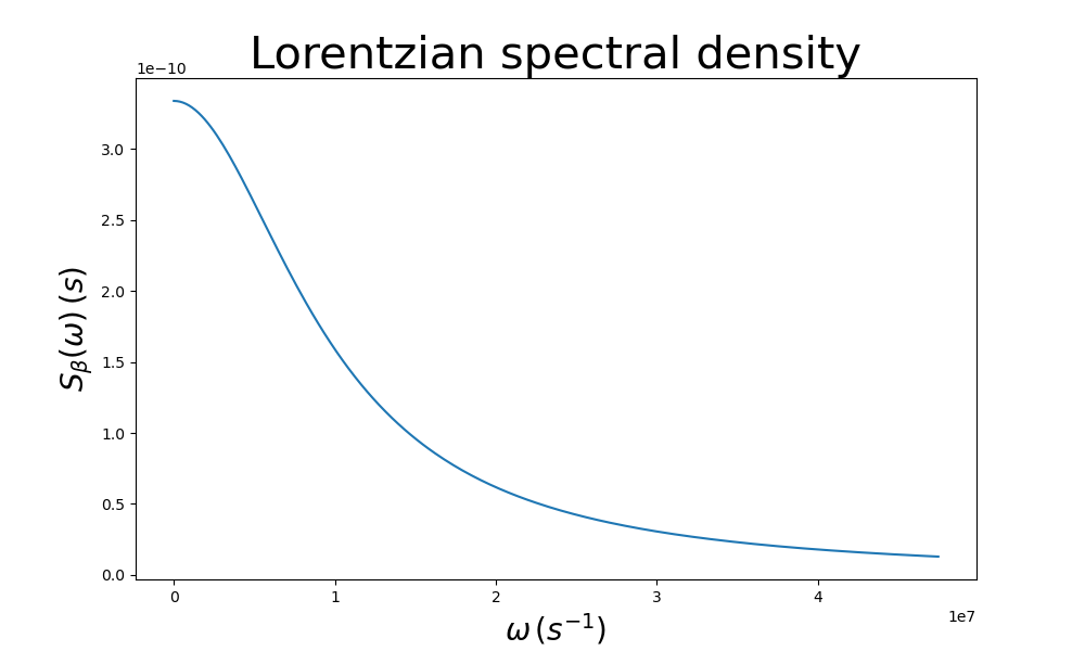
Fig. 2.6.1 Lorentzian

We also generate a random time series with noise coming from the Lorentzian spectrum defined above. This is achieved using the gen_process method.

# Plot time series for the charge noise affecting the gate
# responsible for delta_V.
beta = N.gen_process(times, spectrum, wk, T0)
fig, axes = plt.subplots(1)
fig.set_size_inches((8,5))
axes.plot(times, beta)
axes.set_ylabel(f'$\\beta(t)$', fontsize=20)
axes.set_xlabel('$t \, (s)$', fontsize=20)
plt.show()

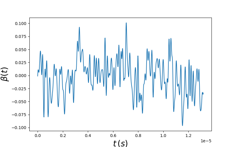
Fig. 2.6.2 beta(t)

We note that because \(\beta\left(t\right)\) is a random time series, the plot produced by running the example should be different from the time series shown here, but vary over similar time scales.

2.7. Simulation including noise

In this final section of the tutorial we will simulate the dynamics of a qubit subject to charge noise. We will assume that this charge noise possesses the Lorentzian spectrum defined above. To perform this simulation, we use the dynamics method of the Noise() object N. This method takes as input the system Hamiltonian, H0, the drive Hamiltonian, delta_V, the modulation frequency of the drive Hamiltonian, omega, the noise spectrum, spectrum, the time scale, T0, the initial state, psi0, an array of times for which we wish to perform the simulation, times, and an operator whose expectation value we wish to obtain at different times—here we chose qutip.sigmaz(). We also specify two optional parameters, vec_omega, the harmonics associated to the spectrum spectrum, and num_runs the number of runs of the simulation [with different time series \(\beta\left(t\right)\)] over which the dynamics should be averaged. Thus, the dynamics functions outputs the expectation value of the operator specified (again, in a frame rotating with frequency omega around the \(z\) axis of the qubit) at each time defined by times, averaged over num_runs number of runs. In other words, the dynamics function solves for the dynamics of a qubit subject to the Hamiltonian \(H\left(t\right)=H_0+\delta V\left[1+\beta\left(t\right)\right]\cos\left(\omega t\right)\), for multiple realizations of the random process \(\beta\left(t\right)\) and computes the expectation value of some operator over these multiple realizations.

In the following block of code we compute \(\braket{\sigma_z\left(t\right)}\) for 1 run and then compute \(\braket{\sigma_z\left(t\right)}\) averaged over 100 runs.

# Simulate dynamic including noise.
num_runs1 = 1 # number of runs to average over
sigz_1run = N.dynamics(H0, delta_V, omega, spectrum, T0, psi0, times,
    qutip.sigmaz(), vec_omega=wk, num_runs=num_runs1)
num_runs2 = 100 # number of runs to average over
sigz_multiruns = N.dynamics(H0, delta_V, omega, spectrum, T0, psi0, times,
    qutip.sigmaz(), vec_omega=wk, num_runs=num_runs2)

The results with and without noise are plotted with

# Plot dynamics
fig, axes = plt.subplots(2)
axes[0].plot(result0.times, qutip.expect(qutip.sigmaz(), result0.states),
    label="Without noise")
axes[0].plot(result0.times, sigz_1run, label="With noise")
axes[1].plot(result0.times, qutip.expect(qutip.sigmaz(), result0.states),
    label="Without noise")
axes[1].plot(result0.times, sigz_multiruns, label="With noise")
# Format Plots
axes[0].set_ylabel(f'$\left< \sigma_z (t) \\right>$', fontsize=20)
axes[1].set_ylabel(f'$\left< \sigma_z (t) \\right>$', fontsize=20)
axes[0].set_xlabel(f'$t \, (s)$', fontsize=20)
axes[1].set_xlabel(f'$t \, (s)$', fontsize=20)
axes[0].set_title(f'num_runs = {num_runs1}')
axes[1].set_title(f'num_runs = {num_runs2}')
axes[0].legend(loc='center left', fontsize=16)
axes[1].legend(loc='center left', fontsize=16)
fig.tight_layout()

plt.show()

which outputs

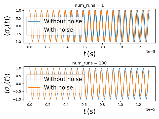
Fig. 2.7.1 dynamics with noise

As can be seen from the top plot where we have a single realization of the dynamics with noise, \(\braket{\sigma_z\left(t\right)}\) is similar (but not identical) to the dynamics in the absence of noise. Once we average \(\braket{\sigma_z\left(t\right)}\) over many realizations of the dynamics (100 in this case), we see that the signal has the same frequency as the dynamics in the absence of noise (the Rabi frequency of the qubit); however, as expected, the amplitude decays over time.

2.8. Full code

__copyright__ = "Copyright 2023, Nanoacademic Technologies Inc."

import numpy as np
from matplotlib import pyplot as plt
from device import constants as ct
import qutip
from qubit import spectra, dynamics, noise

# Copied here are the Hamiltonian and drive for the projected 2 level system
# analyzed in the example `MOS_EDSR.py`. The Hamiltonian and drive are stored in the 
# variables h0 and u on line 145 of `MOS_EDSR.py`.
# System Hamiltonian
h0 = np.array([[1.1128812e-23, 0.00000000e+00],
 [0.00000000e+00, 0.00000000e+00]])
H0 = h0/ct.hbar # Rewrite in units of hbar = 1
# Drive
u = np.array([[-2.03067270e-29, 1.00561612e-27-1.10285789e-37j],
 [1.00561612e-27+1.10285789e-37j, 0.+0.j]])
delta_V = u/ct.hbar # Rewrite in units of hbar = 1

omega = np.absolute(H0[0,0] - H0[1,1]) # qubit frequency
omega_Rabi = np.absolute(delta_V[0,1]) # Rabi frequency on resonance
T_Rabi = 2*np.pi/omega_Rabi # Rabi period

T = 20 * T_Rabi # Total time of the simulations
times = np.linspace(0, T, 1000) # Times at which dynamics are simulated.

# Initialize objects that will handle dynamics and noise.
dyn = dynamics.Dynamics()
N = noise.Noise()

# The Hamiltonian H = H0 + delta_V cos(omega*t) in a frame rotating 
# at frequency omega.
H = dyn.H_RF(H0, delta_V, omega)
# Solve for the dynamics without any noise.
psi0 = qutip.basis(2, 0) # initial state
result0 = qutip.mesolve(H, psi0, times)

# Plot expectation values of sigma_z and sigma_y as a function of time. 
fig, axes = plt.subplots(2)
fig.set_size_inches((8,8))
#<sigma_z (t)>
axes[0].plot(result0.times, qutip.expect(qutip.sigmaz(), result0.states))
#<sigma_y (t)>
axes[1].plot(result0.times, qutip.expect(qutip.sigmay(), result0.states))
# Labels
axes[0].set_ylabel(f'$\left< \sigma_z (t) \\right>$', fontsize=20)
axes[1].set_ylabel(f'$\left< \sigma_y (t) \\right>$', fontsize=20)
axes[0].set_xlabel(f'$t \, (s)$', fontsize=20)
axes[1].set_xlabel(f'$t \, (s)$', fontsize=20)
plt.show()

# Include charge noise which is assumed to affect only the gate which 
# generates the drive delta_V.
# Lorentzian spectrum
S0 = 0.01 # Total power
wc = omega_Rabi # Cutoff frequency
w0 = 0 # Central frequency
# T0 should be much larger than the largest time scale of the problem under consideration.
# Used to properly define the Fourier series of the time series related to the noise. 
T0 = 50 * T_Rabi  # Must take T0 such that 2*pi/T0 << wc to resolve the spectrum
omega_max = 5*wc
wk = np.arange(0, omega_max , 2*np.pi/T0) + w0
spectrum = spectra.lorentz(wk, S0, wc, w0 = w0)

# Plot spectrum
fig, axes = plt.subplots(1)
fig.set_size_inches((10,6))
axes.plot(wk, spectrum)
axes.set_ylabel(f'$S_\\beta(\omega) \, (s)$', fontsize=20)
axes.set_xlabel('$\omega \, (s^{-1})$', fontsize=20)
axes.set_title('Lorentzian spectral density', fontsize=30)
plt.show()

# Plot time series for the charge noise affecting the gate 
# responsible for delta_V.
beta = N.gen_process(times, spectrum, wk, T0)
fig, axes = plt.subplots(1)
fig.set_size_inches((8,5))
axes.plot(times, beta)
axes.set_ylabel(f'$\\beta(t)$', fontsize=20)
axes.set_xlabel('$t \, (s)$', fontsize=20)
plt.show()

# Simulate dynamic including noise.
num_runs1 = 1 # number of runs to average over
sigz_1run = N.dynamics(H0, delta_V, omega, spectrum, T0, psi0, times, 
    qutip.sigmaz(), vec_omega=wk, num_runs=num_runs1)
num_runs2 = 100 # number of runs to average over
sigz_multiruns = N.dynamics(H0, delta_V, omega, spectrum, T0, psi0, times,
    qutip.sigmaz(), vec_omega=wk, num_runs=num_runs2)

# Plot dynamics
fig, axes = plt.subplots(2)
axes[0].plot(result0.times, qutip.expect(qutip.sigmaz(), result0.states), 
    label="Without noise")
axes[0].plot(result0.times, sigz_1run, label="With noise")
axes[1].plot(result0.times, qutip.expect(qutip.sigmaz(), result0.states), 
    label="Without noise")
axes[1].plot(result0.times, sigz_multiruns, label="With noise")
# Format Plots
axes[0].set_ylabel(f'$\left< \sigma_z (t) \\right>$', fontsize=20)
axes[1].set_ylabel(f'$\left< \sigma_z (t) \\right>$', fontsize=20)
axes[0].set_xlabel(f'$t \, (s)$', fontsize=20)
axes[1].set_xlabel(f'$t \, (s)$', fontsize=20)
axes[0].set_title(f'num_runs = {num_runs1}')
axes[1].set_title(f'num_runs = {num_runs2}')
axes[0].legend(loc='center left', fontsize=16)
axes[1].legend(loc='center left', fontsize=16)
fig.tight_layout()

plt.show()