1. Electric dipole spin resonance—Dynamics
1.1. Requirements
1.1.1. Software components
1.1.1.1. Basic Python modules
pathlib
numpy
matplotlib
1.1.1.2. Specific modules
qtcad
qutip
1.1.2. Python script
qtcad/examples/tutorials/MOS_EDSR.py
1.1.3. References
1.2. Briefing
In this tutorial we will simulate the dynamics of an electron subject to the stray magnetic field produced by a micromagnet and the electric field produced by a time-varying voltage applied to a gate (in the vicinity of the electron). The results of the simulation will demonstrate how to drive transitions between the electronic ground- and first-excited (pseudospin) states. This simulation will illustrate how the tools developped within QTCAD® can be used to simulate electric–dipole spin resonance (EDSR) experiments.
It is assumed that the user is familiar with basic Python and has some familiarity with the functionality of the QTCAD code. We also assume some basic familiarity with the QuTiP python library.
The full code may be found at the bottom of this page,
or in MOS_EDSR.py.
1.3. Mesh generation
Before beginning the QTCAD simulation, we use Gmsh to generate a
finite-element mesh on which our problem will be defined. The mesh is
generated from the geometry file
qtcad/examples/tutorials/meshes/MOS_EDSR.geo by running Gmsh.
This can be done in the terminal by running
gmsh MOS_EDSR.geo
within the /examples/meshes directory. This will produce a .msh
file in the same directory as the geometry file. It will also launch
Gmsh and produce an interface where the mesh can be viewed. An image
similar to that given in the figure below
should be produced. See Getting Started for
more information on generating and interfacing with meshes using Gmsh.
Now that the mesh has been generated, we begin the QTCAD simulation.
1.4. Header
First, a header is written to import relevant modules.
import pathlib
import numpy as np
from matplotlib import pyplot as plt

from qtcad.device.mesh3d import Mesh
from qtcad.device import constants as ct
from qtcad.device import materials as mt
from qtcad.device import Device
from qtcad.device.schrodinger import Solver as ssolver
from qtcad.device.schrodinger import SolverParams as SchrodingerSolverParams
from qtcad.device.poisson import Solver as psolver
from qtcad.device.poisson import SolverParams as PoissonSolverParams
from qtcad.device import analysis

from qtcad.device.operators import Gate
from qtcad.qubit import dynamics
import qutip
In the last three lines, we import the modules required specifically to perform a typical EDSR calculation:
Gate: Definition of the
Gateclass. This class is used to modulate the voltage applied to a gate and project the potential energy onto the eigenbasis of the unperturbed system.dynamics: Contains tools to compute and visualize the dynamics of a system. Dynamics are computed using QuTiP.
qutip: QuTiP is a python library that provides tools that can be used to simulate the dynamics of quantum systems.
1.5. Setting up the device
Now that the relevant modules have been imported, we set up the device to be used in this tutorial. We start by importing the mesh on which our problem will be defined. This mesh is the one generated above.
# Mesh
# Path to mesh file
script_dir = pathlib.Path(__file__).parent.resolve()
path_mesh = script_dir / "meshes/" / "MOS_EDSR_example.msh"

# Load the mesh
scaling = 1e-9
mesh = Mesh(scaling, str(path_mesh))
In the figure below we include the labels of the different regions and boundaries labelled using Gmsh (more on this below).
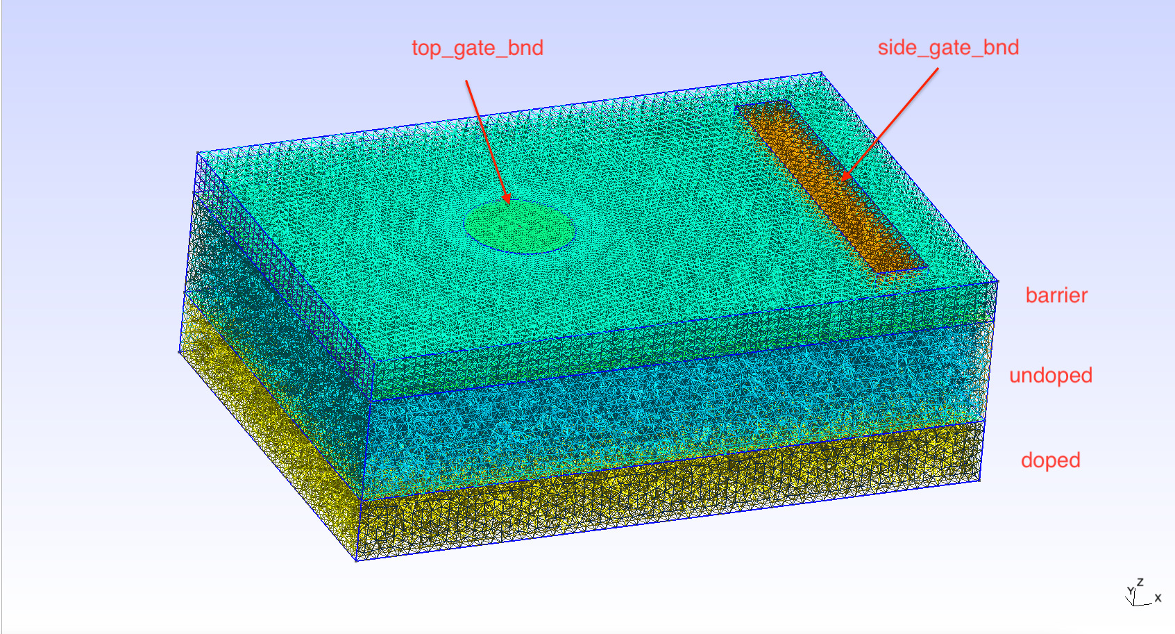
Fig. 1.5.4 Device mesh and its labelled regions and boundaries
Once the mesh is established, we use the
Device constructor to
initialize a Device object from the mesh.
# Create device from mesh and set statistics.
# It is important to set statistics before creating boundaries since
# they determine the boundary values, Failing to do so will produce
# inconsistent results.
# Calculate electronic charge using wavefunctions
d = Device(mesh, conf_carriers="e")
# Analytic approximation to Fermi-Dirac statistics
d.statistics = "FD_approx"
We also specify certain properties of the device (see Poisson and Schrödinger simulation of a nanowire quantum dot for more details.)
Next we specify the material parameters of each region of the device
d,
# Create regions first. The last added region takes priority for
# nodes that are shared by multiple regions.
# Make sure each node is assigned to a region, otherwise default
# (silicon) parameters are used
# Barrier
d.new_region('barrier', mt.SiO2)
# Confined
d.new_region('confined', mt.Si, pdoping=0, ndoping=0)
# The rest
d.new_region('undoped', mt.Si, pdoping=0, ndoping=0)
d.new_region('doped', mt.Si, pdoping=5e18*1e6, ndoping=0)
and the boundary conditions for the device,
# Create boundaries
d.new_ohmic_bnd('bottom')

phi_tg = 1.                             # Top-gate voltage
phi_sg = 0.                             # Side-gate voltage
Ew = mt.Si.chi + mt.Si.Eg/2             # Metal work function
d.new_gate_bnd('top_gate_bnd', phi_tg, Ew)
d.new_gate_bnd('side_gate_bnd', phi_sg, Ew)
In the two blocks of code above, we refer to different regions (first
block) and boundaries (second block) which are labelled using Gmsh.
The image above contains the labels that refer to the different regions
and boundaries of the device. The device contains three layers: a top
green layer, labelled “barrier”, a middle blue layer, labelled
“undoped”, and a lower yellow layer, labelled “doped”. The
new_region() function is used to specify the properties of each
region. The first argument of the new_region() function indicates
which region we are referring to. The second argument specifies the
material the region is composed of. We use this argument to indicate
that the “barrier” region should be made of silicon oxide (SiO2), while
the “undoped” and “doped” regions should be made of silicon. Using the
parameters of the new_region() function we also specify, as the
names suggest, that the “undoped” region is undoped, while the “doped”
region has some p doping. There is an additional region labelled
“confined” made of silicon (more on this region below).
We have also imposed three boundary conditions enforced on three
different surfaces. First, using new_ohmic_bnd(), we enforce an
Ohmic boundary condition applied to the surface labelled “bottom” which
is the bottom face of the device (not visible in the image above). The
other two boundary conditions are specified on the surfaces labelled
“top_gate_bnd” and “side_gate_bnd”. The voltage is specified on each of
these boundaries using the second argument of the new_gate_bnd()
method: 1 V is applied to the top gate, and 0 V are applied to the side
gate. The third argument is used to input the metal work function. The
top gate is used to create a confinement potential which will localize
electrons. Since we expect confinement to occur under the top gate we
define a region labelled “confined” which is more densely meshed under
the top gate (also not visible in the image above). The instructions for
constructing the mesh and labelling the regions using Gmsh can be found
in MOS_EDSR.geo.
Thus, using Gmsh, we have defined a MOS (metal top gate, silicon oxide barrier, silicon channel) qubit device. The side gate will be used to electrically drive transitions between different (pseudospin) states of an electron confined to the region of space under the top gate.
For more information on generating meshes and interfacing with QTCAD, see Getting Started, Poisson and Schrödinger simulation of a nanowire quantum dot, and Schrödinger equation for a quantum dot.
1.6. Solving the Poisson equation
Now that the device along with the boundary conditions are defined, we can solve for eigenstates of our system using the core functionalities of QTCAD. This will be achieved by first solving for the electrostatics of the problem using the Poisson solver. This solver will yield a potential which can later be used by the QTCAD Schrödinger solver to solve the system Hamiltonian and find any bound eigenstates.
We start by initializing the Poisson solver with the device d as an
input and then using the solve method to solve for the
conduction-band edge throughout the device.
ps = psolver(d)
ps.solve() # Solve the Poisson equation using default parameters
Then, we convert the conduction-band edge to a potential using the
set_V_from_phi method.
# Convert the electric potential from the Poisson solver into a potential
# for the Schrödinger solver
d.set_V_from_phi()
The potential will be stored in an attribute of the device, d.V.
It will be the potential in the Hamiltonian solved by the Schrödinger
solver.
1.7. Setting the magnetic field
The main goal of this tutorial is to introduce users to EDSR simulations using
the operators module.
The specific EDSR setup that we will consider uses a micromagnet and the associated position-dependent stray magnetic field to achieve an effective electron spin–orbit coupling. This coupling between spin and orbital degrees of freedom allows for time-varying electric fields (rather than magnetic fields) to drive Rabi oscillations. While intrinsic spin–orbit couplings can also enable the possibility of driving EDSR, the strength/speed of the transitions relying on intrinsic spin–orbit coupling will be material dependent and fixed. In contrast, using the effective spin–orbit coupling generated from a micromagnet allows for the possibility of EDSR even in materials where the intrinsic spin–orbit coupling is weak (e.g. for electrons in silicon). Furthermore, this technique has been employed successfully in multiple devices. See e.g.:
The first step to simulating EDSR in the presence of a micromagnet using QTCAD is to define the magnetic fields throughout the device.
def Bfield(x, y, z):
   B0 = 0.6 # homogeneous magnetic field (T)
   b = 0.3 * 1e6 # magnetic-field gradient (T/micron)

   return np.array([B0, 0, b*x])

d.set_Bfield(Bfield)
This is achieved by passing the function Bfield to the setter
set_Bfield.
The magnetic field is taken to have a constant homogeneous piece which points
along the \(x\) direction and has a magnitude \(B_0=0.6\,\mathrm{T}\).
We also assume the micromagnet will generate a stray field along
the \(z\) direction which varies linearly over the \(x\) coordinate
(magnitude: \(b=0.3 \textrm{ T}\cdotp\mu\textrm{m}^{-1}\)).
This position-dependent magnetic field couples
the ground orbital level with excited orbital levels with opposite spin,
similar to a spin–orbit coupling, as can be seen from
Eq. (12.1) of the Quantum control theory section.
Note
Calling
set_Bfield
here may produce a warning about orbital magnetic
effects not being considered in a spatially varying B field. Since we are
not interested in these effects here, this warning may be safely ignored.
Because a magnetic field has been set, the associated Zeeman term will be included in the Hamiltonian when we solve the Schrödinger equation. However, because the magnetic field is inhomogenous, the following warning will be printed indicating that we cannot include orbital magnetic effects in our simulation.
UserWarning: Cannot include orbital magnetic effects for varying B field.
1.8. Solving the Schrödinger equation
We configure the Schrödinger solver to solve for the six lowest-energy
(confined) eigenstates of the system using the Schrödinger
SolverParams module.
Once the solver is initialized with the proper parameters, we run the
solve method.
These steps are implemented using:
# Configure the Schrödinger solver
params_schrod = SchrodingerSolverParams()
num_states = 6
params_schrod.num_states = num_states # Number of energy levels to consider
params_schrod.tol = 1e-12
ss = ssolver(d, solver_params=params_schrod)

ss.solve() # Solve the Schrödinger equation
Note
This may trigger a warning about the value of the effective g factor in
silicon dioxide, which is not defined in the
materials module. By default, the value in
silicon will be used. Here, this warning may be safely ignore because most
of the electron wave function will indeed reside in silicon. In other
circumstances, it may be useful to manually the g factor using the
set_param method
of the Material class.
We can also plot the densities associated with the four eigenfunctions
using the analysis module and the plot_slices method
states = np.sum(np.abs(d.eigenfunctions)**2, axis=2)
# Plot eigenstates
analysis.plot_slices(mesh, states[:, 0], x=0, y=0, z=30*scaling,
   title="Ground-state density")
analysis.plot_slices(mesh, states[:, 1], x=0, y=0, z=30*scaling,
   title="First-excited-state density")
analysis.plot_slices(mesh, states[:, 2], x=0, y=0, z=30*scaling,
   title="Second-excited-state density")
analysis.plot_slices(mesh, states[:, 3], x=0, y=0, z=30*scaling,
   title="Third-excited-state density")
analysis.plot_slices(mesh, states[:, 4], x=0, y=0, z=30*scaling,
   title="Fourth-excited-state density")
analysis.plot_slices(mesh, states[:, 5], x=0, y=0, z=30*scaling,
   title="Fifth-excited-state density")
The resulting plots are shown below.
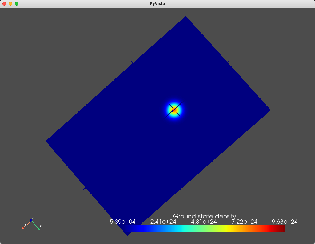
Fig. 1.8.1 Ground state

Fig. 1.8.2 First excited state

Fig. 1.8.3 Second excited state
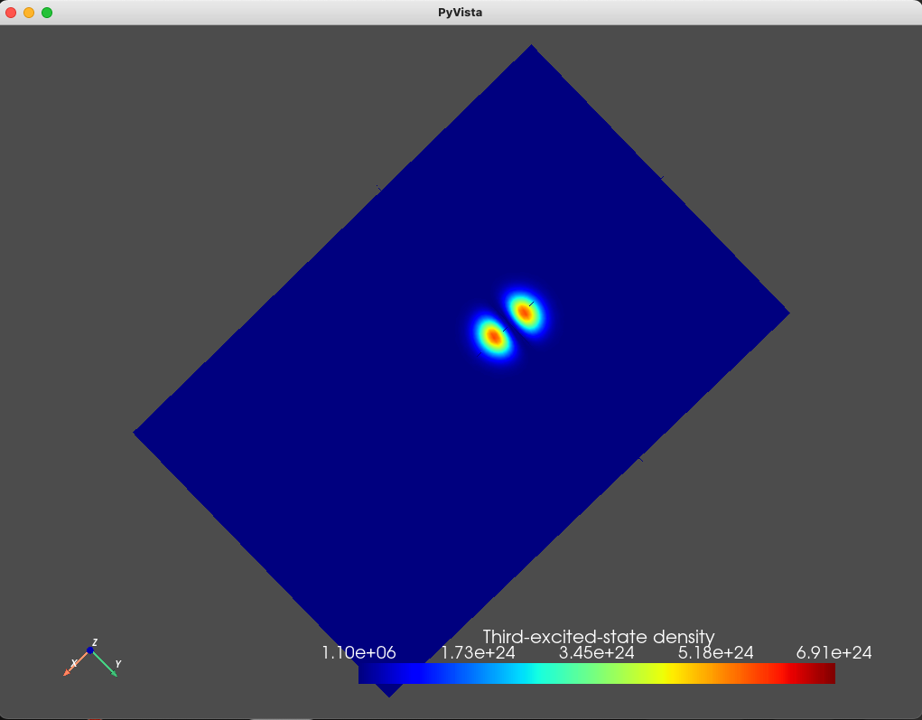
Fig. 1.8.4 Third excited state
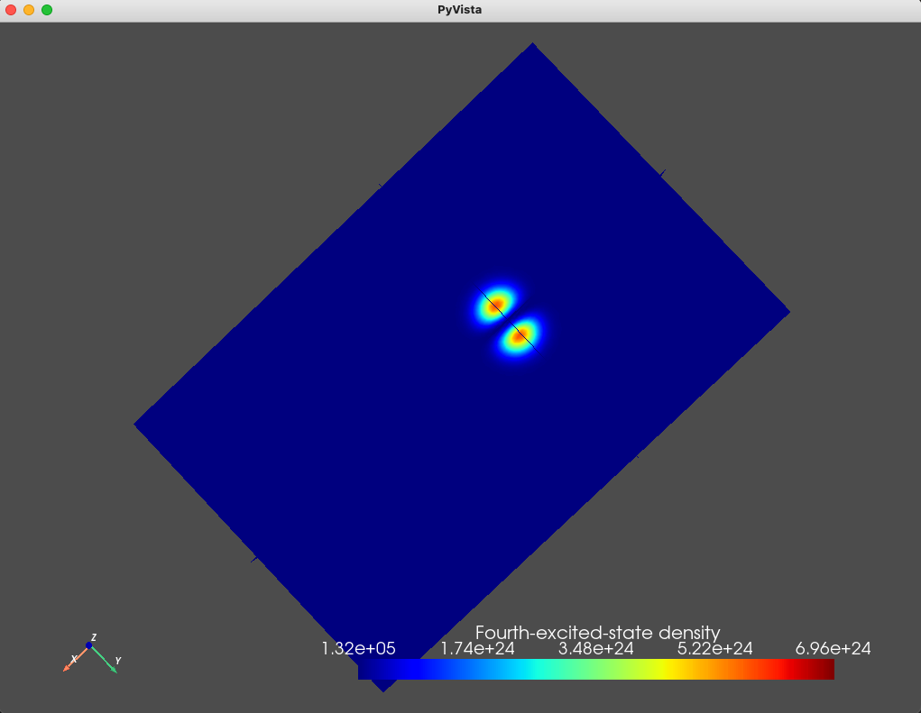
Fig. 1.8.5 Fourth excited state
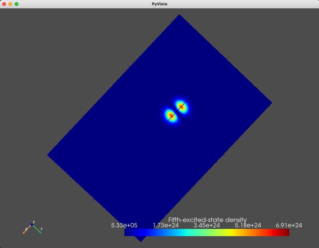
Fig. 1.8.6 Fifth excited state
As can be seen from these figures, the electronic wavefunctions are confined to a compact region of space located beneath the top gate. We also print the eigenenergies (in \(\textrm{eV}\) units) using
# Energies
d.print_energies()
which will output
Energy levels (eV)
[0.76791229 0.76798176 0.79342199 0.79345759 0.79349146 0.79352715]
As we expect, the ground- and first- excited states have the same orbital character (but different spin character) which is reflected in the identical electronic density. These are split in energy by the Zeeman effect. Moreover, since the top gate is circular, in the absence of any magnetic field, we expect a fourfold degeneracy: a twofold orbital degeneracy and a twofold spin degeneracy (similar to a 2D harmonic oscillator). We see that the second-, third-, fourth-, and fifth-excited states all have a single node, consistent with all four states having the same orbital character.
Up until now, we have described a typical QTCAD simulation (accounting for the Zeeman effect). For more details look at the other tutorials demonstrating the core features of QTCAD (see Poisson and Schrödinger simulation of a nanowire quantum dot). The remainder of this tutorial will be about simulating EDSR.
1.9. Computing the matrix representation of the drive
The next step is to calculate the (time-dependent) potential energy matrix in
the system eigenbasis (which will include spin due to the Zeeman effect).
This can be achieved using a Gate
operator.
The Gate constructor has three inputs, i.e. the device under consideration
(d), the name of the gate we wish to apply these voltages to
('side_gate_bnd'), and the voltage we wish to apply (V).
We also pass in, via the keyword argument params, solver parameters for the
non-linear Poisson solver used by the
Gate operator to compute the
operator matrix.
gate_biases = np.linspace(0, 2, num=6)
gate = 'side_gate_bnd'
UU = np.zeros((len(gate_biases), num_states, num_states), dtype=complex)

# Parametrize Poisson solver (inside Gate operator)
gate_params = PoissonSolverParams()
gate_params.tol = 1e-3

for i, V in enumerate(gate_biases):
   # Apply V to gate and compute the potential energy operator matrix
   G = Gate(d, gate, V, params=gate_params)
   UU[i, :, :] = G.get_operator_matrix()
The
get_operator_matrix
method of G computes the matrix representation of the perturbation
associated potential–energy operator for the given voltage applied to the side
gate in the basis defined by the
energies and the
eigenfunctions attributes of
d.
These matrices are \(6 \times 6\) where the indices run over the
eigenfunctions of d.
For every value of V, the associated matrix is stored in UU.
1.10. Observing Rabi oscillations
A general calculation of the dynamics of the system could be performed as follows:
The times \(t_i\) at which we wish to know the state of the system are determined.
The potentials that are applied to the side gate are determined using some drive function, \(\varphi^\textrm{bias}_i=\varphi^\textrm{bias}\left(t_i\right)\).
The potential energy matrix, \(\delta V_i\), is determined for each of these \(\varphi^\textrm{bias}_i\) [using the
solve()function]. This matrix is given byUU[i,:,:].We solve for the dynamics of the problem using the array based scheme in QuTiP.
In our specific calculation, the problem is greatly simplified because the potential energy matrix is a linear function of the applied voltage \(\varphi^\textrm{bias}\). To see this, we plot the \(0\to 1\) matrix element of the potential energy matrix, \(\delta V_{01}\), as a function of \(\varphi^\textrm{bias}\) (the voltage applied to the side gate):
# The potential energy matrix is a linear function of the applied voltage
fig= plt.figure()

# Plot - 01 matrix element
ax1 = fig.add_subplot(111)
ax1.plot(gate_biases, np.abs(np.real(UU[:, 0, 1])/ct.e), '.-', label="Real")
ax1.plot(gate_biases, np.abs(np.imag(UU[:, 0, 1])/ct.e), '.-', label="Imaginary")
ax1.set_xlabel(r'$\varphi^\mathrm{bias}$', fontsize=20)
ax1.set_ylabel(r'$\delta V_{01}(\varphi^\mathrm{bias})$ (eV)', fontsize=20)
ax1.grid()
ax1.legend()
fig.tight_layout()
plt.show()
The output is shown below.
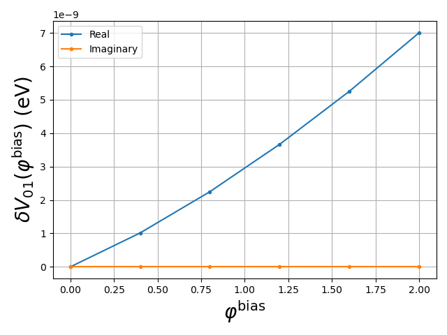
Fig. 1.10.1 Real and imaginary parts of an element of the potential energy matrix as function of applied voltage
To within a reasonable approximation, this matrix element is a linear function
of \(\varphi^\textrm{bias}\).
Plotting the other matrix elements in a similar way, it can be verified
that the entire potential energy matrix, in this example, is
reasonably well-approximated by a linear function of the applied voltage.
Thus, any modulation of the voltage applied to the side gate will result in a
similar (scaled) modulation of the potential energy matrix.
Here, we will consider a sinusoidal modulation of the potential energy matrix
generated by a sinusoidal modulation of the voltage applied to the side gate.
The largest applied voltage (the amplitude of \(2 \, \mathrm{V}\))
corresponds to the potential energy matrix stored in UU[-1], i.e. the last
potential energy matrix.
We will use this matrix to linearly interpolate the potential energy matrices
for all applied potentials in an EDSR simulation.
# Use the fact that the perturbing potential is a linear function of the
# applied voltage.
delta_V = UU[-1]
As mentioned above, H0 is the system Hamiltonian in the eigenbasis
and is therefore diagonal. The eigenenergies can be printed (in eV
units) using
# System Hamiltonian in the eigenbasis is diagonal
E = d.energies
E = E - (E[0]) # Go into frame rotating at ground-state frequency

# Create Hamiltonian
H0 = np.diagflat(E)
print(f'evals (eV): {np.diagonal(H0)/ct.e}')
The eigenergies are:
evals (eV):[0.00000000e+00 6.94605817e-05 2.55096841e-02 2.55452442e-02 2.55791447e-02 2.56147048e-02]
where, as mentioned above, the energies are evaluated with respect to
the ground state energy. While the ground state and first excited state
are separated by tens of μeV, these two states are separated from the
others by tens of meV. Therefore, it should be a good approximation to
consider the first 2 levels as a well isolated 2 level system.
Consequently, it is well justified to simplify the problem by projecting
the operators describing the system onto the subspace spanned by the
ground and first excited states. Using this simplification along with
the fact that the potential energy matrix is linear in
\(\varphi^\textrm{bias}\), we can
analyze the dynamics of an electron under the influence of a sinusoidal
voltage applied to the side gate using a single method of a Dynamics
object, transition_2_levels():
# Simple EDSR calculation. The calculation is performed by projecting onto
# the relevant 2 dimensional subspace. Here we are studying transitions
# from the ground state (j=0) to the first excited state (i=1). The optional
# parameter plot is set to true to visualize the results.
dyn = dynamics.Dynamics()
result, h0, u, omega0, omega_rabi = dyn.transition_2_levels(1, 0, H0,
   delta_V, plot=True, npts=4000)
The transition_2_levels() method implements the theory described in the
subsection called A simple scenario: a driven two-level system under the rotating-wave approximation in the Quantum control theory section.
This method has four arguments: the index of the state that we chose as
the up state \(\ket{\uparrow}\) (i.e. 1), the index of the state that we chose as the down
state \(\ket{\downarrow}\) (i.e. 0), the system hamiltonian (H0), and the potential energy
matrix amplitude (delta_V). The convention chosen in
transition_2_levels() is one where the Pauli \(z\) operator is
\(\sigma_z = \ket{\uparrow}\bra{\uparrow} - \ket{\downarrow}\bra{\downarrow}\)
and it assumes that the initial state in the
calculation of the dynamics of the system will be \(\ket{\downarrow}\). This method has
five outputs:
a
resultQuTiP object that contains information about the dynamics,h0, the projected two-level system Hamiltonian,u, the projected two-level potential energy matrix,omega0, the resonance frequency, andomega_rabi, the Rabi frequency of the transition.
Furthermore, by setting the plot parameter to True, a plot of
the projections onto the \(\ket{\downarrow}\) state
(\(P_{\downarrow}\left(t\right)=\left|\braket{\downarrow|\psi\left(t\right)}\right|^2\))
and the \(\ket{\uparrow}\) state
(\(P_{\uparrow}\left(t\right)=\left|\braket{\uparrow|\psi\left(t\right)}\right|^2\))
as a function of time will be produced using QuTiP.
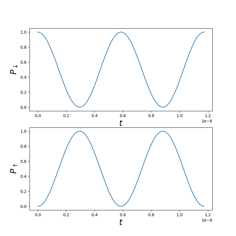
Fig. 1.10.2 Two-level dynamics
The domain of this plot is 2 Rabi cycles. The resonance frequency, Rabi frequency, and Rabi cycles are calculated based on the standard theory for Rabi oscillations (see e.g. the Rabi cycle Wikipedia aritcle).
We note that the method transition_2_levels() has other optional
inputs: the driving frequency, omega (taken to be the resonance
frequency by default), the time for which the dynamics should be
evaluated, T (taken to be 2 Rabi cycles by default), and the number
of equally spaced time points for which the calculation will be
performed, npts (taken to be 1000 by default).
1.11. More accurate calculation
While the procedure above allowed us to see Rabi oscillations using a single function call, we emphasize that we expect this to be a valid approach only in the limit where we have a well-isolated two-level system. In this section, we will anyalyze the same problem, however, this time, without projecting onto a two-level subspace. This section of the tutorial requires some basic understanding of the QuTiP Python library.
The first step is to initialize the system and potential energy
Hamiltonian matrices. Here, we will write all energies in units of
\(\hbar\). We also initialize the full time dependent Hamiltonian H.
This initialization is done in the format required to calculate dynamics
using QuTiP. In particular, we make use of the Qobj class.
# We simulate the dynamics of
# an electron initialized in the ground state subject to a modulating voltage
# applied to the side gate without projecting onto a two-dimensional subspace.
# This section of the code requires a basic understanding of the QuTip library
H0 = qutip.Qobj(H0/ct.hbar) # system Hamiltonian in units of hbar
# Reset the zero of energy (ground state has E!=0).
np.fill_diagonal(delta_V, delta_V.diagonal()-delta_V[0,0])
delta_V = qutip.Qobj(delta_V/ct.hbar) # potential energy matrix amplitude in units of hbar
H = [H0, [delta_V, 'cos(omega0*t)']] # Full Hamiltonian - sinusoidal modulation of delta_V
In the above code snippet, we are shifting the diagonal matrix elements of
delta_V by a constant amount. This shift amounts to neglecting some terms
proportional to the identity and will allow for the computation
performed by QuTiP below to converge more efficiently. Remark that in contrast
with the transition_2_levels() method, the current approach does not
imply any RWA and will thus contain fast oscillating terms.
In this example, we drive the voltage applied to the side gate
sinusoidally at the resonance frequency of the transition we wish to
observe. In this case we are interested in a transition between the
ground and first-excited states. The resonance frequency has already
been calculated as an output of transition_2_levels().
args = {'omega0': omega0}
For more information on the format of these variables, see the QuTiP documentation. Next, we initialize the system in the ground state using:
psi0 = qutip.basis(6, 0) # initialize in the ground state
and we use QuTiP’s mesolve function to solve for the dynamics of a
system under the influence of the Hamiltonian H for a time
2*T_Rabi [which is also be computed using one of the outputs of
transition_2_levels()].
T_Rabi = 2* np.pi / omega_rabi # Rabi cycle in the two-level limit
# array of times for which the solver should store the state vector
tlist = np.linspace(0, 2*T_Rabi, 500000)
print("Computing Rabi oscillations beyond two-dimensional subspace.")
print("This may take several minutes.")
result = qutip.mesolve(
    H,
    psi0,
    tlist,
    c_ops=[],
    e_ops=[],
    args=args,
    options={"progress_bar": "tqdm"},
)
In contrast to the two-level example presented above, many more points
are required for the QuTiP mesolve calculation to converge
(~ 450,000 to be precise). Therefore, this calculation takes much longer
to complete, in comparison to the one presented above. Once it is
complete, we can plot the probability to be in each of the 6 states as a
function of time. First, we use the EDSR module to obtain the
projectors onto each of the states, and then plot the expectation values
of these projectors using Matplotlib.
# using the EDSR module to get projectors onto the 6 basis states
Proj = dyn.projectors(6)
# Plot projections onto each state.
fig, axes = plt.subplots(2,3)
for i in range(2):
    for j in range(3):
        axes[i,j].plot(tlist, qutip.expect(Proj[3*i+j], result.states))
        axes[i,j].set_xlabel(r'$t$', fontsize=20)
        axes[i,j].set_ylabel(f'$P_{3*i+j}$', fontsize=20)
fig.tight_layout()
plt.show()
The resulting plot is
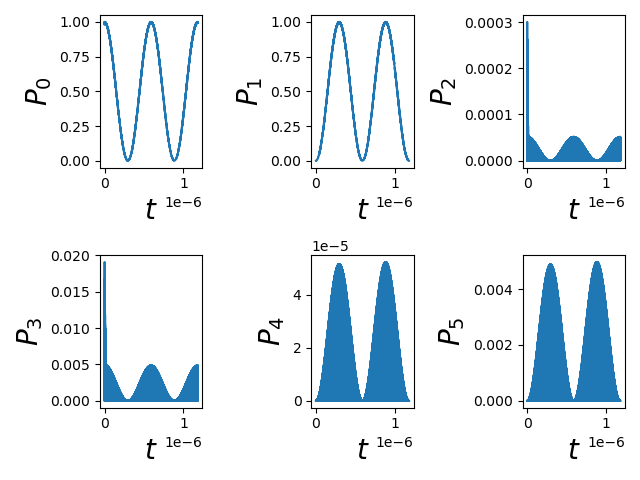
Fig. 1.11.1 Multi-level dynamics
Comparing this figure to the one presented above, we can see that the projections onto the ground and excited states as a function of time are quite similar. Therefore, in this case, the projection onto the 2 dimensional subspace seems to have been justified (there is very little leakage to the other states). However, this will not always be the case. In particular we expect the more thorough analysis presented in this section of the tutorial to be more important when a 2 level system of interest is not properly isolated.
In Electric dipole spin resonance—Noise, we will study how voltage fluctuations at a gate (arising, say, from charge noise) can affect the visibility of Rabi oscillations.
Warning
Because of the extreme difference in timescales between leakage dynamics
(which evolves over nanoseconds or less) and Rabi oscillations (which
occur over hundreds of nanoseconds or over microseconds), in a given
simulation, an exhaustive convergence analysis with respect to the
QuTiP time resolution and solver tolerance
(controlled by the atol, rtol, and nsteps solver
Options)
may be necessary.
Unless this convergence is
achieved, leakage oscillations may vary significantly between
machines and operating systems.
1.12. Full code
__copyright__ = "Copyright 2022-2026, Nanoacademic Technologies Inc."

import pathlib
import numpy as np
from matplotlib import pyplot as plt
from qtcad.device.mesh3d import Mesh
from qtcad.device import constants as ct
from qtcad.device import materials as mt
from qtcad.device import Device
from qtcad.device.schrodinger import Solver as ssolver
from qtcad.device.schrodinger import SolverParams as SchrodingerSolverParams
from qtcad.device.poisson import Solver as psolver
from qtcad.device.poisson import SolverParams as PoissonSolverParams
from qtcad.device import analysis
from qtcad.device.operators import Gate
from qtcad.qubit import dynamics
import qutip

# Mesh
# Path to mesh file
script_dir = pathlib.Path(__file__).parent.resolve()
path_mesh = script_dir / "meshes/" / "MOS_EDSR_example.msh"

# Load the mesh
scaling = 1e-9
mesh = Mesh(scaling, str(path_mesh))

# Create device from mesh and set statistics.
# It is important to set statistics before creating boundaries since
# they determine the boundary values, Failing to do so will produce
# inconsistent results.
# Calculate electronic charge using wavefunctions
d = Device(mesh, conf_carriers="e")
# Analytic approximation to Fermi-Dirac statistics
d.statistics = "FD_approx"

# Create regions first. The last added region takes priority for
# nodes that are shared by multiple regions.
# Make sure each node is assigned to a region, otherwise default
# (silicon) parameters are used
# Barrier
d.new_region("barrier", mt.SiO2)
# Confined
d.new_region("confined", mt.Si, pdoping=0, ndoping=0)
# The rest
d.new_region("undoped", mt.Si, pdoping=0, ndoping=0)
d.new_region("doped", mt.Si, pdoping=5e18 * 1e6, ndoping=0)

# Create boundaries
d.new_ohmic_bnd("bottom")

phi_tg = 1.0  # Top-gate voltage
phi_sg = 0.0  # Side-gate voltage
Ew = mt.Si.chi + mt.Si.Eg / 2  # Metal work function
d.new_gate_bnd("top_gate_bnd", phi_tg, Ew)
d.new_gate_bnd("side_gate_bnd", phi_sg, Ew)

ps = psolver(d)
ps.solve()  # Solve the Poisson equation using default parameters

# Convert the electric potential from the Poisson solver into a potential
# for the Schrödinger solver
d.set_V_from_phi()


def Bfield(x, y, z):
    B0 = 0.6  # homogeneous magnetic field (T)
    b = 0.3 * 1e6  # magnetic-field gradient (T/micron)

    return np.array([B0, 0, b * x])


d.set_Bfield(Bfield)


# Configure the Schrödinger solver
params_schrod = SchrodingerSolverParams()
num_states = 6
params_schrod.num_states = num_states  # Number of energy levels to consider
params_schrod.tol = 1e-12
ss = ssolver(d, solver_params=params_schrod)

ss.solve()  # Solve the Schrödinger equation

states = np.sum(np.abs(d.eigenfunctions) ** 2, axis=2)
# Plot eigenstates
analysis.plot_slices(
    mesh, states[:, 0], x=0, y=0, z=30 * scaling, title="Ground-state density"
)
analysis.plot_slices(
    mesh, states[:, 1], x=0, y=0, z=30 * scaling, title="First-excited-state density"
)
analysis.plot_slices(
    mesh, states[:, 2], x=0, y=0, z=30 * scaling, title="Second-excited-state density"
)
analysis.plot_slices(
    mesh, states[:, 3], x=0, y=0, z=30 * scaling, title="Third-excited-state density"
)
analysis.plot_slices(
    mesh, states[:, 4], x=0, y=0, z=30 * scaling, title="Fourth-excited-state density"
)
analysis.plot_slices(
    mesh, states[:, 5], x=0, y=0, z=30 * scaling, title="Fifth-excited-state density"
)

# Energies
d.print_energies()

gate_biases = np.linspace(0, 2, num=6)
gate = "side_gate_bnd"
UU = np.zeros((len(gate_biases), num_states, num_states), dtype=complex)

# Parametrize Poisson solver (inside Gate operator)
gate_params = PoissonSolverParams()
gate_params.tol = 1e-3

for i, V in enumerate(gate_biases):
    # Apply V to gate and compute the potential energy operator matrix
    G = Gate(d, gate, V, params=gate_params)
    UU[i, :, :] = G.get_operator_matrix()

# The potential energy matrix is a linear function of the applied voltage
fig = plt.figure()

# Plot - 01 matrix element
ax1 = fig.add_subplot(111)
ax1.plot(gate_biases, np.abs(np.real(UU[:, 0, 1]) / ct.e), ".-", label="Real")
ax1.plot(gate_biases, np.abs(np.imag(UU[:, 0, 1]) / ct.e), ".-", label="Imaginary")
ax1.set_xlabel(r"$\varphi^\mathrm{bias}$", fontsize=20)
ax1.set_ylabel(r"$\delta V_{01}(\varphi^\mathrm{bias})$ (eV)", fontsize=20)
ax1.grid()
ax1.legend()
fig.tight_layout()
plt.show()

# Use the fact that the perturbing potential is a linear function of the
# applied voltage.
delta_V = UU[-1]

# System Hamiltonian in the eigenbasis is diagonal
E = d.energies
E = E - (E[0])  # Go into frame rotating at ground-state frequency

# Create Hamiltonian
H0 = np.diagflat(E)
print(f"evals (eV): {np.diagonal(H0) / ct.e}")

# Simple EDSR calculation. The calculation is performed by projecting onto
# the relevant 2 dimensional subspace. Here we are studying transitions
# from the ground state (j=0) to the first excited state (i=1). The optional
# parameter plot is set to true to visualize the results.
dyn = dynamics.Dynamics()
result, h0, u, omega0, omega_rabi = dyn.transition_2_levels(
    1, 0, H0, delta_V, plot=True, npts=4000
)

# We simulate the dynamics of
# an electron initialized in the ground state subject to a modulating voltage
# applied to the side gate without projecting onto a two-dimensional subspace.
# This section of the code requires a basic understanding of the QuTip library
H0 = qutip.Qobj(H0 / ct.hbar)  # system Hamiltonian in units of hbar
# Reset the zero of energy (ground state has E!=0).
np.fill_diagonal(delta_V, delta_V.diagonal() - delta_V[0, 0])
delta_V = qutip.Qobj(
    delta_V / ct.hbar
)  # potential energy matrix amplitude in units of hbar
H = [
    H0,
    [delta_V, "cos(omega0*t)"],
]  # Full Hamiltonian - sinusoidal modulation of delta_V

args = {"omega0": omega0}

psi0 = qutip.basis(6, 0)  # initialize in the ground state

T_Rabi = 2 * np.pi / omega_rabi  # Rabi cycle in the two-level limit
# array of times for which the solver should store the state vector
tlist = np.linspace(0, 2 * T_Rabi, 500000)
print("Computing Rabi oscillations beyond two-dimensional subspace.")
print("This may take several minutes.")
result = qutip.mesolve(
    H,
    psi0,
    tlist,
    c_ops=[],
    e_ops=[],
    args=args,
    options={"progress_bar": "tqdm"},
)

# using the EDSR module to get projectors onto the 6 basis states
Proj = dyn.projectors(6)
# Plot projections onto each state.
fig, axes = plt.subplots(2, 3)
for i in range(2):
    for j in range(3):
        axes[i, j].plot(tlist, qutip.expect(Proj[3 * i + j], result.states))
        axes[i, j].set_xlabel(r"$t$", fontsize=20)
        axes[i, j].set_ylabel(f"$P_{3 * i + j}$", fontsize=20)
fig.tight_layout()
plt.show()