1. Poisson and Schrödinger simulation of a GAAFET
1.1. Requirements
1.1.1. Software components
QTCAD
Gmsh
1.1.2. Geometry file
qtcad/examples/tutorials/meshes/gaafet.geo
1.1.3. Python script
qtcad/examples/tutorials/gaafet.py
1.1.4. References
1.2. Briefing
In this tutorial, we explain how to perform a basic electrostatic
calculation for conduction electrons at equilibrium in a gate-all-around
field-effect transistor (GAAFET). It is assumed that the user is
familiar with basic Python. It is also assumed that the user has access
to the Gmsh geometry file describing the GAAFET device to simulate.
Geometry files for all the QTCAD tutorials are stored in the folder
examples/tutorials/meshes.
The full code may be found at the bottom of this page,
or in qtcad/examples/tutorials/gaafet.py.
Do not hesitate to look into the API source code for detailed descriptions of the inputs and outputs of each class, method, or function used in the tutorials. The source code also contains documentation for many other useful features not described here.
1.3. Mesh generation
The mesh is generated from the
geometry file qtcad/examples/tutorials/meshes/gaafet.geo by running Gmsh.
This can be done in the terminal with
gmsh gaafet.geo
This wil produce a .msh file in the same directory as the geometry
file. See Arbitrary geometry definition with Gmsh for more information about
interfacing with Gmsh.
1.4. Setting up the device and solving the electrostatic problem
1.4.1. Header
A header is first written to import relevant modules from the QTCAD Device simulator.
from qtcad.device import constants as ct
from qtcad.device.mesh3d import Mesh
from qtcad.device import io
from qtcad.device import analysis
from qtcad.device import materials as mt
from qtcad.device import Device
from qtcad.device.poisson import Solver as PoissonSolver
from qtcad.device.schrodinger import Solver as SchrodingerSolver
from qtcad.device.poisson import SolverParams as PoissonSolverParams
from qtcad.device.schrodinger import SolverParams as SchrodingerSolverParams

import pathlib
This imports modules (or classes within modules) that are necessary to the execution of the code that follows. Here is a brief description of what each of these modules is responsible for.
constants: Universal physical constants (elementary charge, Planck’s constant, etc.).
mesh3d: Definition of the 3D Mesh class, which stores information about the position of mesh points, their connectivity (definition of elements, physical regions and boundaries).
io: Functions to save and load certain variables into and from files.
analysis: Functions useful for processing and analysis of simulation outcomes; e.g. producing 3D plots and linecuts.
materials: Objects describing each material supported by QTCAD. Here, a material is an object whose attributes are the material parameters such as the effective mass tensor or permittivity.
device: Definition of the Device class, which is central to all simulations done with QTCAD. A device object stores the value of all physical parameters (effective mass, permittivity, dopant densities, etc.) and variables (electric potential, carrier densities) at each element or mesh point.
poisson: Contains the non-linear Poisson solver which will be used below to calculate the electric potential and band-edge profile of the device.
schrodinger: Contains the Schrödinger solver which will be used below to find the envelope functions and eigenenergies of single conduction electrons confined in the conduction band edge profile found by solving Poisson’s equation.
Remark that the poisson and
schrodinger modules both contain
Solver and SolverParams classes. While the Solver classes
contain algorithms needed to solve the corresponding equations, the
SolverParams classes may be used to control parameters of these
algorithms.
1.4.2. Input parameters
# Define some device parameters
Vgs = 0.5 # Gate-source bias
Ew = mt.Si.chi + mt.Si.Eg/2 # Metal work function
Ltot = 20e-9 # Device height in m
radius = 2.5e-9 # Device radius in m
The first line defines the gate-to-source bias \(V_{GS} = V_G - V_S\),
which is applied at the device boundary wrapped around the oxide shell.
The next line defines the work function of the metal forming the gate
contact surrounding the transistor. This work function is chosen to be
equal to the work function of intrinsic silicon at zero temperature.
Finally, the last two parameters are the device height and radius; these
quantities are not used as inputs to the simulation (the geometry being
entirely defined in gaafet.geo), but
are defined for later plotting purposes.
In addition to the device parameters above, paths to various input and output files are defined, which will be used below.
# Paths to mesh file and output files
script_dir = pathlib.Path(__file__).parent.resolve()
path_mesh = script_dir / "meshes" / "gaafet.msh"
path_hdf5 = script_dir / "output" / "gaafet.hdf5"
path_vtu = script_dir / "output" / "gaafet.vtu"
path_energies = script_dir / "output" / "gaafet_energies.txt"
path_linecuts_z = script_dir / "output" / "gaafet_linecuts_z.txt"
path_linecuts_x = script_dir / "output" / "gaafet_linecuts_x.txt"
1.4.3. Defining the mesh
The mesh is defined by loading the mesh file produced by Gmsh and setting units of length
# Load the mesh
scaling = 1e-9
mesh = Mesh(scaling, str(path_mesh))
Note the two arguments of the constructor of the Mesh class: scaling
and str(path_mesh). While str(path_mesh) is simply the string
pointing at the mesh file to use, scaling indicates a number by
which all coordinates in the mesh file should be multiplied. Since the
code uses SI units, the value chosen here (1e-9) indicates that lengths
in the mesh file are nanometers.
The mesh may also be displayed using:
# Plot the mesh
mesh.show()
This will call the Visualization ToolKit (VTK) through its Python wrapper (PyVista) to produce a 3D representation of the mesh, like this:
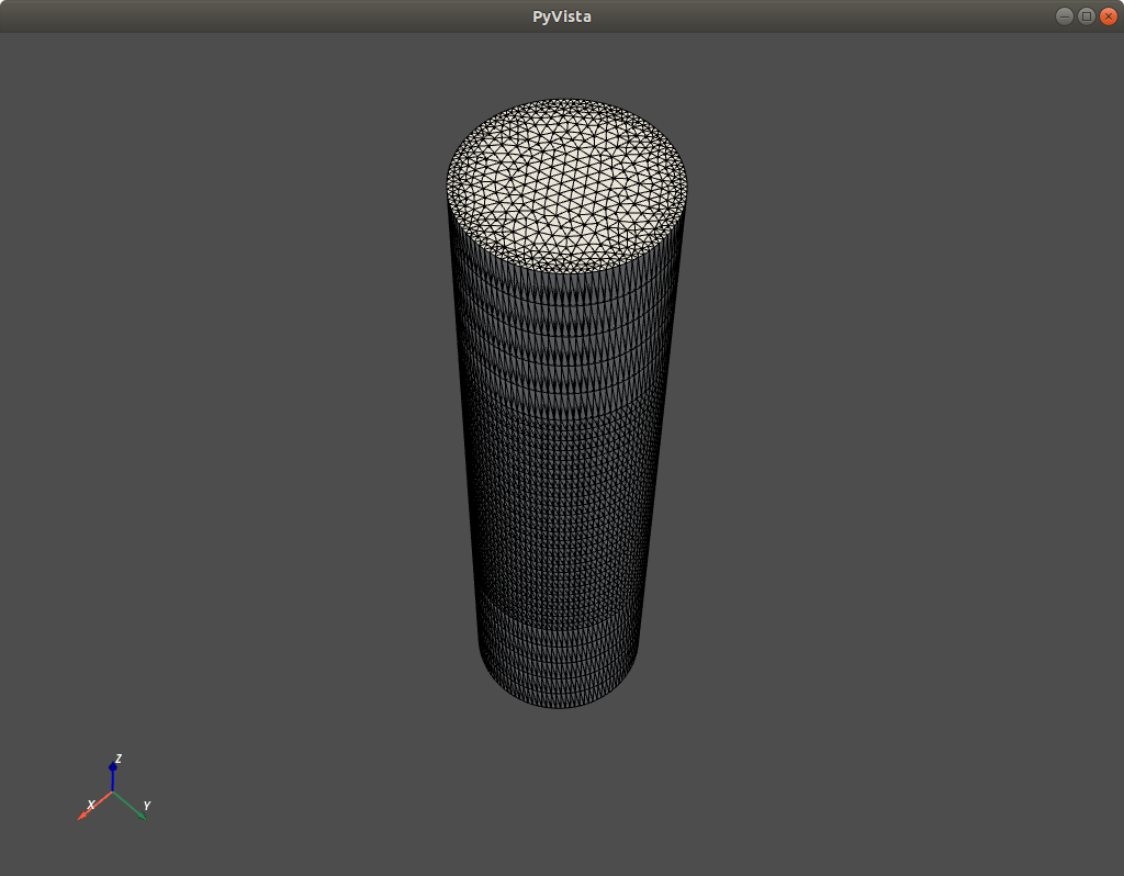
Fig. 1.4.1 Mesh illustration
1.4.4. Creating the device
The device to simulate is then initialized on the mesh defined above:
# Create device from mesh and set statistics.
# It is important to set statistics before creating boundaries since
# they determine the boundary values. Failing to do so will produce
# inconsistent results.
d = Device(mesh)
d.statistics = "FD_approx"  # Analytic approximation to Fermi-Dirac statistics (default)
The first line calls the constructor of the device class with the mesh
object as an argument. The second line specifies which statistical model
is used to calculate classical carrier densities at equilibrium. Choices
are "MB" (Maxwell–Boltzmann), "FD" (Fermi–Dirac), and "FD_approx"
(approximate Fermi–Dirac). The first choice ("MB") is simple and
efficient but inaccurate, and leads to poor convergence at strong doping
densities. The second choice ("FD") uses Fermi–Dirac statistics by
calculating Fermi–Dirac integrals numerically. This is the most accurate
choice, but imposes a significant computational overhead. The third
choice ("FD_approx", which is also the default value) considers
Fermi–Dirac statistics, but uses analytic approximations of the
Fermi–Dirac integrals that provide a relative error \(\leq 0.4 \%\) on carrier
densities to speed up calculations. This reduced accuracy is rarely a
limitation in practice. For more information on analytic approximations
of the Fermi–Dirac integrals, see
Gao et al. J. Appl. Phys. 114, 164302 (2013).
Bednarczyk and J. Bednarczyk, Phys. Lett. A 64, 409 (1978).
Van Halen and D. L. Pulfrey. J. Appl. Phys. 57, 5271 (1985).
Note
Since we have not specified any temperature here, the device temperature
will take its default value of \(300~\mathrm{K}\). Temperature may be set with the
set_temperature
method of the Device class.
Note that in all QTCAD simulations, temperature is assumed to be uniform.
Note
Upon instantiation of the Device object, the following warning is printed:
The attribute conf_carriers of the device object was not specified; conf_carriers will be set to 'e'.
The Device attribute conf_carriers specifies which charge carriers
(electrons or holes) are to be treated quantum-mechanically by the various
quantum solvers of QTCAD, e.g., the Schrödinger equation solver. By default,
conf_carriers is set to 'e', meaning that electrons but not holes
are treated quantum-mechanically. This warning may be turned off by
instantiating the Device object d through d = Device(mesh, conf_carriers="e").
1.4.5. Specifying physical regions and boundaries
It is now time to specify the value of device parameters (doping density, effective mass, permittivity, etc.) at each point of the mesh over which the device is build. This may be done explicitly for each node of the mesh; however this approach is tedious and produces code that is prone to bugs and difficult to read. A better way is to leverage physical volumes and surfaces defined in the geometry file to define regions and boundaries.
Regions are a collection of elements that belong to a given 3D physical group. A physical group is a set of elements associated with an integer or string label in the geometry file. It is possible to define regions based on physical groups, and specify a material for such a region. In the present example, this is done as follows
# Create regions first.
# Make sure each element is assigned to a region, otherwise default
# (silicon) parameters are used
d.new_region('channel_ox',mt.SiO2)
d.new_region('source_ox',mt.SiO2)
d.new_region('drain_ox',mt.SiO2)
d.new_region('channel', mt.Si)
d.new_region('source', mt.Si, pdoping=5e20*1e6, ndoping=0)
d.new_region('drain', mt.Si, pdoping=5e20*1e6, ndoping=0)
The first three lines define the oxide that surrounds the channel,
source, and drain regions, respectively, using their string labels
defined in the geometry file (and stored in the .msh file). The
material used is silicon dioxide (mt.SiO2). The last three lines define the
semiconductor (silicon) regions, and set the source and drain to be
positively doped with a doping density of \(5 \times 10^{20} \textrm{ cm}^{-3}\).
Remark: When writing geometry files, it is important to make sure that all elements in a given mesh belong to one and only one region. If an element belongs to two or more regions at the same time, an exception will be raised. If an element does not belong to any region, then its nodes will be given default properties (those of intrinsic silicon).
In addition to 3D physical groups (physical volumes), Gmsh supports 2D physical groups (physical surfaces), which also associate certain two-dimensional elements to a label. These may be leveraged to define boundaries as follows:
# Then create boundaries
d.new_ohmic_bnd('source_bnd')
d.new_ohmic_bnd('drain_bnd')
d.new_gate_bnd('gate_bnd',Vgs,Ew)
This creates two Ohmic boundaries located at the ends of the source and drain regions, respectively, along with a gate boundary at the surface that wraps around the channel. As in defining regions, the first argument is the string label used in Gmsh. For the gate boundary, the second argument is the applied potential (which is added to the built-in potential calculated internally using the relevant physical model). The method that creates a gate boundary also requires a third argument, i.e. the metal work function.
1.4.6. Creating and running the Poisson solver
Once the device and its parameters are defined, a non-linear Poisson
solver can be instantiated and executed. In the header of the current
file, we have imported the
Solver
class of the
poisson
module. We have also imported the
SolverParams class of the
poisson
module, which enables us to configure the Poisson solver. A
solver object is then instantiated with
# Create and configure the non-linear Poisson solver
params_poisson = PoissonSolverParams()
params_poisson.tol = 1e-5 # Convergence threshold (tolerance) for the error
s = PoissonSolver(d, solver_params=params_poisson)
The first line instantiates an object used to define the parameters of the non-linear Poisson solver. The second line sets the error tolerance on the electric potential in volts, i.e. the error threshold below which the non-linear Poisson self-consistent loop is considered to have converged. The last line instantiates the Poisson solver, with parameters specified using the two previous lines.
Note that the solver is instantiated with the device d as input
argument, enabling the solver to correctly calculate the potentials and
charge densities appropriate to the geometry, mesh, materials, and
doping levels stored in this object. This also indicates that results of
the calculations will be stored in this device.
Once the non-linear Poisson solver is configured, the problem is simply solved with
# Self-consistent solution
s.solve()
This will launch the following self-consistent loop: 1. The electric
potential is set to the default initial guess (charge-neutral
configuration). 2. The equilibrium electron and hole distribution
resulting from this electric potential is calculated following the
carrier statistics model chosen above ("FD_approx"). 3. The electric
potential is calculated again by solving the Poisson equation resulting
from the charge distribution corresponding to appropriate electron,
hole, and ionized dopant concentrations. 4. Steps 2 and 3 are iterated
until the potential varies by less than the tolerance between successive
iterations.
1.5. Saving and visualizing results
1.5.1. Spatially-dependent variables
We may save the value of spatially-dependent variables (carrier densities) at each mesh point as follows
# To save throughout the device: n, p, phi, EC, EV
arrays_dict = {"n": d.n/1e6, "p": d.p/1e6, "phi": d.phi,
    "EC": d.cond_band_edge()/ct.e, "EV": d.vlnce_band_edge()/ct.e}
io.save(str(path_hdf5), arrays_dict)
The first line creates a dictionary of arrays to save, i.e. a set of
objects labeled by strings. Each object is an array giving the value of
a variable at each local node in the mesh. Variables considered here
are, respectively, the electron density, the hole density, the electric
potential, the conduction band edge, and the valence band edge (we
convert units of density into \(\textrm{cm}^{-3}\), and units of energy
into \(\textrm{eV}\)). Note that the format in which data is to be saved is
determined automatically from the extension of the file in the input path, here
.hdf5, as dictated by the path_hdf5 variable.
The second line saves all these quantities in the file whose path is
path_hdf5. Specific variables stored in a Python array (e.g. the
electric potential) may subsequently be loaded from this data file
simply with
# A given variable may then be loaded with
phi = io.load(str(path_hdf5), "phi")
As will be seen later, it is possible to visualize results directly in
QTCAD. However, for more extensive 3D data visualization with a
Graphical User Interface, it is useful to export the data into a
.vtu file, which may then be loaded in
ParaView, a free, open-source, and
multi-platform data analysis and visualization application. Saving into
.vtu format may be done with:
# These variables may also be saved in vtu format for external visualization
io.save(str(path_vtu), arrays_dict, mesh)
When saving into .vtu format, it is important to specify the mesh,
since the files will contain information about the geometry. In
addition, because ParaView does not easily handle distances with very
small numerical values (~1e-9), distances in the .vtu file are
rescaled to be expressed with respect to a chosen unit of length, which
may be set using the keyword argument length_unit. Available values
for this argument are 'nm', 'um', 'mm', and 'm'. The
default unit of length in output .vtu files is 'nm'.
1.5.2. Linecuts
For 3D devices, it is often useful to consider variables along specific linecuts. The following code block shows how to save the variables defined above along two linecuts: one that corresponds to the symmetry axis (along \(z\)) of the GAAFET, and one that cuts through the device along the direction perpendicular to the symmetry axis in the middle of the channel.
# Linecuts along z with x=y=0 for the same quantities
# Save n, p and phi throughout the device and along z axis
arrays = [d.n, d.p, d.phi]
array_names = ["n", "p", "phi"]
analysis.save_linecut(str(path_linecuts_z), mesh, arrays,
    (0,0,0), (0,0,Ltot), array_names=array_names)

# Linecuts along x with z=L/2 and y=0 for the same quantities
analysis.save_linecut(str(path_linecuts_x), mesh, arrays,
    (-radius,0,Ltot/2.), (radius,0,Ltot/2.), array_names=array_names)
1.5.3. Plotting linecuts of the results
The data saved in .vtu format may easily be imported and plotted in
ParaView. In addition, for 2D plots, it is straightforward to use
the standard Python library Matplotlib. However, QTCAD also includes
some simple visualization functions that are useful to plot results on
the fly.
For example, a linecut of the electric potential may be directly plotted with:
# Plot linecut of the potential along the z axis
analysis.plot_linecut(mesh,d.phi,(0,0,0),(0,0,Ltot),
    title='Electric potential (V)')
which produces:
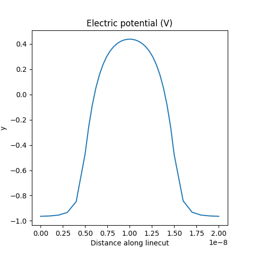
Fig. 1.5.1 Electric potential
The following code also enables to plot the band diagram across a given linecut
# Plot band diagram
analysis.plot_bands(d, (0,0,0), (0,0,Ltot))
The result is
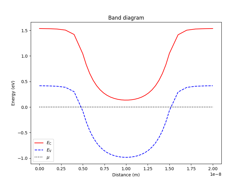
Fig. 1.5.2 Band diagram
1.6. Solving Schrödinger’s equation
1.6.1. Setting up the confinement potential and the Schrödinger solver
We first specify which charge carrier (electrons: 'e', holes:
'h') shall be treated as confined in this simulation. Looking at the
above band diagram, it is clear that the electrons are the confined
carriers since there is a potential well in the conduction band edge for
electrons, but a potential barrier in the valence band edge for holes.
In addition, we must retrieve the confinement potential for the chosen charge carrier resulting from the electric potential calculated with the Poisson solver.
The above two actions are completed with
# Calculate the confinement potential from the electric potential
# found above, and set the confined carriers to be electrons
# The confinement potential is stored in d.V
d.conf_carriers = 'e'
d.set_V_from_phi()
The next step is to instantiate the Schrödinger solver and its parameters. This is very similar to what was done above for the Poisson solver.
# Then instantiate the Schrodinger solver and its parameters
params_schrod = SchrodingerSolverParams()
params_schrod.tol = 1e-5        # Tolerance on energies in eV
params_schrod.num_states = 5    # Number of states to consider
s = SchrodingerSolver(d, solver_params=params_schrod)
In the first line, we instantiate a
SolverParams
object appropriate to
Schrödinger solvers. The second line sets the tolerance on energies in
electron-volts. The third line specifies the number of eigenstates and
energies to consider (starting from and including the ground state) in
the diagonalization of the device Hamiltonian. The fourth line
instantiates the Schrödinger solver based on the device object (which
contains the confinement potential in the attribute d.V) and on the
solver parameters.
1.6.2. Solving Schrödinger’s equation and viewing results
We then solve Schrödinger’s equation with
# Solve Schrodinger's equation
s.solve()
As before, the results of the calculation are stored in relevant device
attributes, here d.energies and d.eigenfunctions. The attribute
d.energies contains all the eigenenergies in SI units in ascending
order from the ground state. The attribute d.eigenfunctions is a 2D
array whose first index (rows) corresponds to global nodes in the mesh,
and whose second index (columns) corresponds to the eigenenergies, in
ascending order.
The energy levels may be printed on the screen and saved in a text file using
# Output and save energy levels
d.print_energies()
d.save_energies(str(path_energies))
For the current example, this yields
Energy levels (eV)
[0.54798018 0.61320023 0.68496648 0.7631776  0.84786669]
The energies are expressed with respect to the Fermi level (set to zero throughout the device at equilibrium).
In addition, we may compute and print the geometric properties of the
quantum dot using the analyze_dot
function of the analysis module:
# Get and print the quantum-dot geometric properties
dot_props = analysis.analyze_dot(d, verbose=True)
These properties are stored in the dictionary dot_props. If the
verbose keyword argument is set to True, the function will also
print the properties on the screen. For the current example, this yields:
--------------------------------------------------------------------------------
Geometric properties of the quantum dot:
--------------------------------------------------------------------------------
position        :  [ 2.70608902e-13 -4.88703648e-13  9.99954680e-09]
std             :  [5.84702875e-10 5.84499147e-10 9.32973459e-10]
size            :  [2.33881150e-09 2.33799659e-09 3.73189383e-09]
--------------------------------------------------------------------------------
Here, the length units are in meters. Definitions of dot position and size are
given in the API reference of the
analyze_dot function.
1.7. Visualizing results in 3D
For detailed and flexible 3D visualization, it is best to export the
quantities to be visualized in .vtu format (see above), and open
them in ParaView (see Visualizing QTCAD quantities with ParaView).
However, it is often convenient to produce quick and dirty plots
directly from the QTCAD Python API at the end of a simulation. This may
be done through functions stored in the analysis module, which wrap
relevant PyVista functions.
For example, density plots of each variable of interest may be displayed on orthogonal planar slices inside the device with:
# Plot p and phi (with n and p converted to cm^-3)
# on orthogonal planar slices inside the device
analysis.plot_slices(mesh,d.p/1e6,title='p (cm^-3)')
analysis.plot_slices(mesh,d.phi,title='phi (V)')
Above, we multiply the densities by 1e-6 to convert from SI units to CGS.
The output for the hole density looks like this:
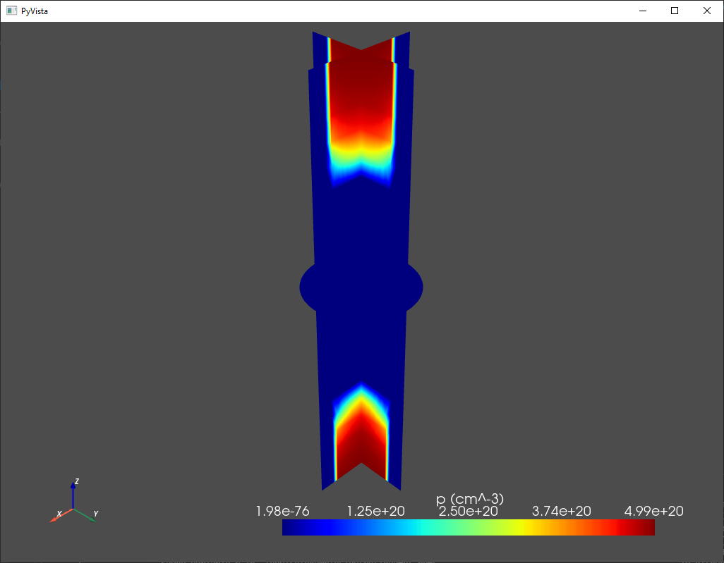
Fig. 1.7.1 Classical hole density
We may then plot the first few electron envelope functions with
# Plot ground and first few excited state wavefunctions along the same slices
analysis.plot_slices(mesh,d.eigenfunctions[:,0],title="Ground state")
analysis.plot_slices(mesh,d.eigenfunctions[:,1],title="First excited state")
analysis.plot_slices(mesh,d.eigenfunctions[:,2],title="Second excited state")
This results in the three following figures.
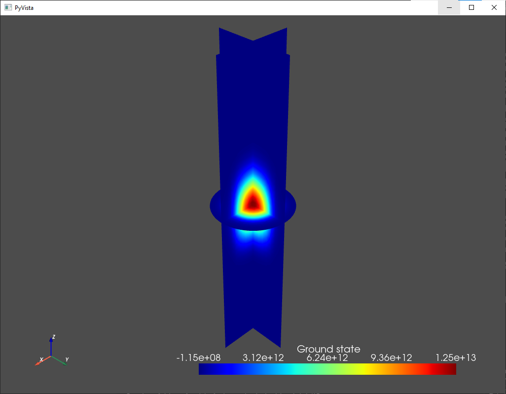
Fig. 1.7.2 Ground state
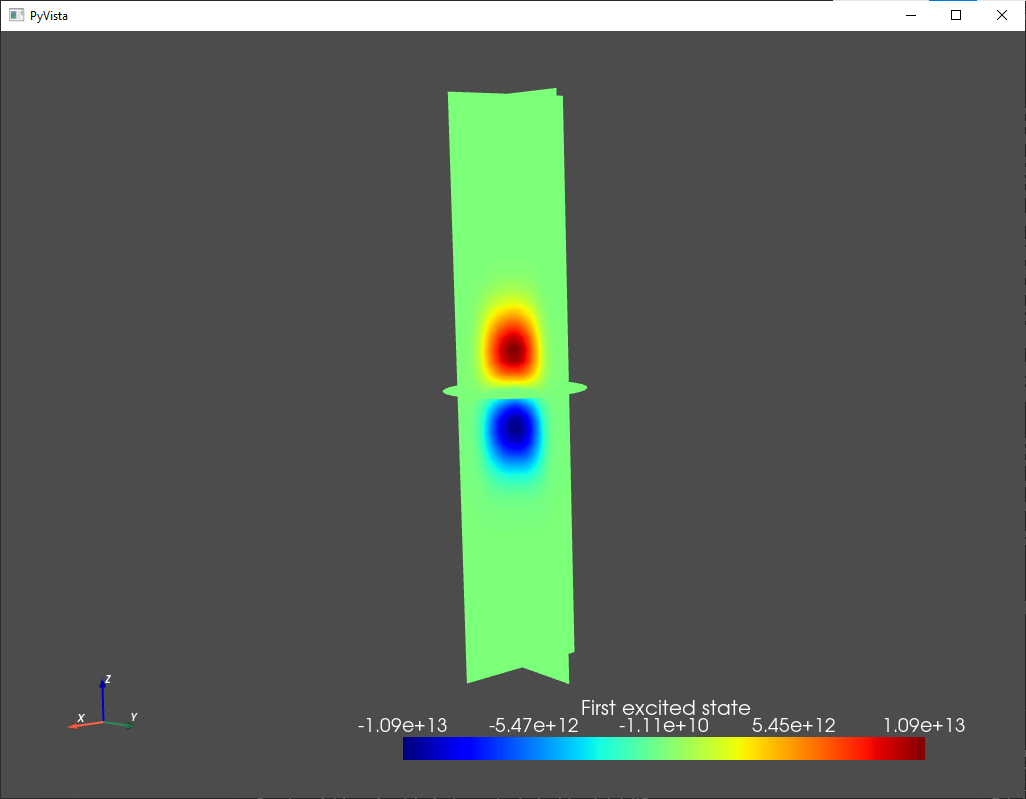
Fig. 1.7.3 First excited state
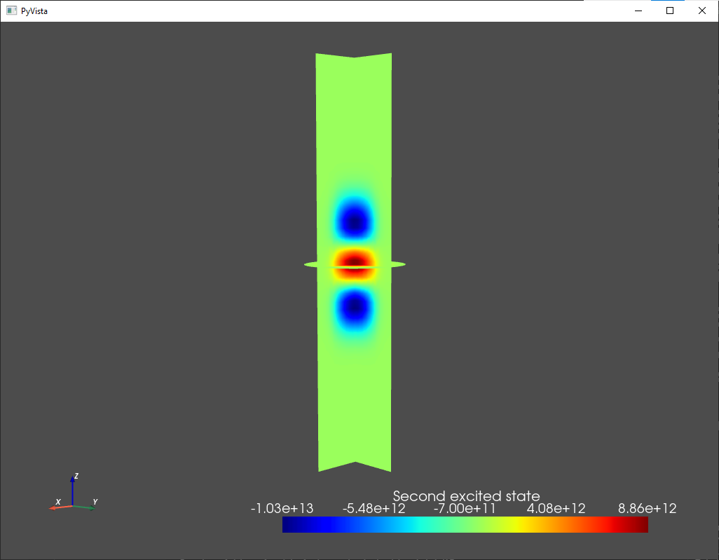
Fig. 1.7.4 Second excited state
In Quantum transport—Master equation, we will see how to use the confinement potential obtained here to define a many-body problem, and compute a charge-stability diagram for quantum transport by sequential tunneling through the GAAFET system.
1.8. Full code
__copyright__ = "Copyright 2024, Nanoacademic Technologies Inc."

from qtcad.device import constants as ct
from qtcad.device.mesh3d import Mesh
from qtcad.device import io
from qtcad.device import analysis
from qtcad.device import materials as mt
from qtcad.device import Device
from qtcad.device.poisson import Solver as PoissonSolver
from qtcad.device.schrodinger import Solver as SchrodingerSolver
from qtcad.device.poisson import SolverParams as PoissonSolverParams
from qtcad.device.schrodinger import SolverParams as SchrodingerSolverParams
import pathlib

# Define some device parameters
Vgs = 0.5 # Gate-source bias
Ew = mt.Si.chi + mt.Si.Eg/2 # Metal work function
Ltot = 20e-9 # Device height in m
radius = 2.5e-9 # Device radius in m

# Paths to mesh file and output files
script_dir = pathlib.Path(__file__).parent.resolve()
path_mesh = script_dir / "meshes" / "gaafet.msh"
path_hdf5 = script_dir / "output" / "gaafet.hdf5"
path_vtu = script_dir / "output" / "gaafet.vtu"
path_energies = script_dir / "output" / "gaafet_energies.txt"
path_linecuts_z = script_dir / "output" / "gaafet_linecuts_z.txt"
path_linecuts_x = script_dir / "output" / "gaafet_linecuts_x.txt"

# Load the mesh
scaling = 1e-9
mesh = Mesh(scaling, str(path_mesh))

# Plot the mesh
mesh.show()

# Create device from mesh and set statistics.
# It is important to set statistics before creating boundaries since
# they determine the boundary values. Failing to do so will produce
# inconsistent results.
d = Device(mesh)
d.statistics = "FD_approx"  # Analytic approximation to Fermi-Dirac statistics (default)

# Create regions first.
# Make sure each element is assigned to a region, otherwise default
# (silicon) parameters are used
d.new_region('channel_ox',mt.SiO2)
d.new_region('source_ox',mt.SiO2)
d.new_region('drain_ox',mt.SiO2)
d.new_region('channel', mt.Si)
d.new_region('source', mt.Si, pdoping=5e20*1e6, ndoping=0)
d.new_region('drain', mt.Si, pdoping=5e20*1e6, ndoping=0)

# Then create boundaries
d.new_ohmic_bnd('source_bnd')
d.new_ohmic_bnd('drain_bnd')
d.new_gate_bnd('gate_bnd',Vgs,Ew)

# Create and configure the non-linear Poisson solver
params_poisson = PoissonSolverParams()
params_poisson.tol = 1e-5 # Convergence threshold (tolerance) for the error
s = PoissonSolver(d, solver_params=params_poisson)

# Self-consistent solution
s.solve()

# To save throughout the device: n, p, phi, EC, EV
arrays_dict = {"n": d.n/1e6, "p": d.p/1e6, "phi": d.phi,
    "EC": d.cond_band_edge()/ct.e, "EV": d.vlnce_band_edge()/ct.e}
io.save(str(path_hdf5), arrays_dict)

# A given variable may then be loaded with
phi = io.load(str(path_hdf5), "phi")

# These variables may also be saved in vtu format for external visualization
io.save(str(path_vtu), arrays_dict, mesh)

# Linecuts along z with x=y=0 for the same quantities
# Save n, p and phi throughout the device and along z axis
arrays = [d.n, d.p, d.phi]
array_names = ["n", "p", "phi"]
analysis.save_linecut(str(path_linecuts_z), mesh, arrays,
    (0,0,0), (0,0,Ltot), array_names=array_names)

# Linecuts along x with z=L/2 and y=0 for the same quantities
analysis.save_linecut(str(path_linecuts_x), mesh, arrays,
    (-radius,0,Ltot/2.), (radius,0,Ltot/2.), array_names=array_names)

# Plot linecut of the potential along the z axis
analysis.plot_linecut(mesh,d.phi,(0,0,0),(0,0,Ltot),
    title='Electric potential (V)')

# Plot band diagram
analysis.plot_bands(d, (0,0,0), (0,0,Ltot))

# Calculate the confinement potential from the electric potential
# found above, and set the confined carriers to be electrons
# The confinement potential is stored in d.V
d.conf_carriers = 'e'
d.set_V_from_phi()

# Then instantiate the Schrodinger solver and its parameters
params_schrod = SchrodingerSolverParams()
params_schrod.tol = 1e-5        # Tolerance on energies in eV
params_schrod.num_states = 5    # Number of states to consider
s = SchrodingerSolver(d, solver_params=params_schrod)

# Solve Schrodinger's equation
s.solve()

# Output and save energy levels
d.print_energies()
d.save_energies(str(path_energies))

# Get and print the quantum-dot geometric properties
dot_props = analysis.analyze_dot(d, verbose=True)

# Plot p and phi (with n and p converted to cm^-3)
# on orthogonal planar slices inside the device
analysis.plot_slices(mesh,d.p/1e6,title='p (cm^-3)')
analysis.plot_slices(mesh,d.phi,title='phi (V)')

# Plot ground and first few excited state wavefunctions along the same slices
analysis.plot_slices(mesh,d.eigenfunctions[:,0],title="Ground state")
analysis.plot_slices(mesh,d.eigenfunctions[:,1],title="First excited state")
analysis.plot_slices(mesh,d.eigenfunctions[:,2],title="Second excited state")