6. Band alignment in heterostructures
6.1. Requirements
6.1.1. Software components
QTCAD
Gmsh
6.1.2. Geometry file
qtcad/examples/tutorials/meshes/band_alignment.geo
6.1.3. Python script
qtcad/examples/tutorials/band_alignment.py
6.1.4. References
6.2. Briefing
Band alignment is crucial in defining barriers and wells for electrons and holes in semiconductor devices. It thereby significantly impacts the electrostatics and transport properties of semiconductor devices. This tutorial introduces various methods for modeling band alignment in QTCAD and explores the impact of band alignment on carrier confinement in heterostructures.
QTCAD has three main approaches for modeling band alignment:
Anderson’s rule, wherein band offsets are computed by aligning vacuum levels across heterojunctions; band offsets are thereby parametrized by the electron affinities and bandgaps of the relevant semiconductor materials. Anderson’s rule provides a quick and simple estimate of band offsets, but ignores, among other things, charge transfer across heterojunctions, which may significantly affect band offsets.
Band alignment from atomistic simulations, wherein band offsets are computed from first-principles atomistic simulations, thereby providing greater accuracy than Anderson’s rule. The
materialsmodule of QTCAD contains parameters to compute such band offsets for GaAs/AlGaAs and Si/SiGe heterojunctions, which were computed using Nanoacademic Technologies’ density-functional theory package RESCU.Custom band alignments, which allows for user-defined band offsets.
As vehicles to this tutorial, we consider three common heterostructures:
AlGaAs/GaAs/AlGaAs (Groups III-V, electron well),
SiGe/Si/SiGe (Group-IV, electron well),
SiGe/Ge/SiGe (Group-IV, hole well).
Specifically, we compute band diagrams for these heterostructures using the three band alignment methods mentioned above. In addition, we demonstrate the impact of band alignment on bound state wavefunction obtained via QTCAD’s Schrödinger equation solver. Finally, we show how to sweep Ge content \(x\) in the relaxed \(\text{Si}_{1-x}\text{Ge}_{x}\) barriers of a SiGe/Si/SiGe heterostructure to tabulate conduction-band and valence-band offsets as a function of Ge composition \(x\), which is a common design task, e.g. when optimizing tunnel barriers and strain.
6.3. Mesh generation
As usual, the mesh is generated from the geometry file by running Gmsh as follows.
gmsh examples/tutorials/meshes/band_alignment.geo
In the Gmsh GUI, clicking Options > Geometry, we may modify the GUI
parameters to show the physical lines corresponding to each region of the
device.
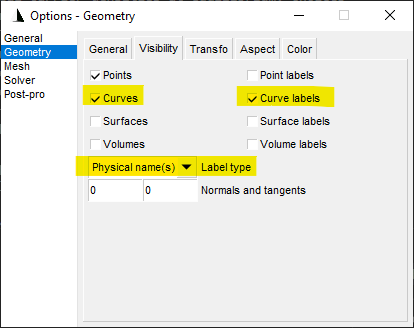
Fig. 6.3.1 Options in Gmsh visualization
This results in
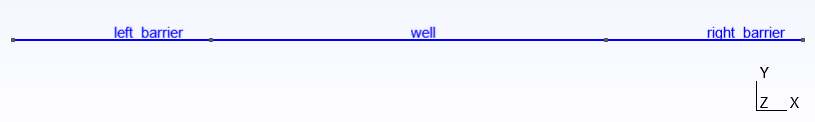
Fig. 6.3.2 1D mesh
The physical lines are labelled left_barrier, well, and
right_barrier. We reuse the same 1D mesh for all three investigated
heterostructures. Each heterostructure is specified by the material assigned to
left_barrier, well, and right_barrier.
6.4. Anderson’s rule, RESCU-based band alignment, and Schrödinger solver in an AlGaAs/GaAs/AlGaAs heterostructure
6.4.1. Header
A header is first written to import relevant modules from the QTCAD device
package.
import numpy as np
from matplotlib import pyplot as plt
from pathlib import Path

from qtcad.device import constants as ct
from qtcad.device.mesh1d import Mesh
from qtcad.device import Device
from qtcad.device import materials as mt
from qtcad.device import analysis as an
from qtcad.device.schrodinger import Solver
6.4.2. Defining the mesh
The QTCAD mesh is defined by loading the mesh file produced by Gmsh and setting the units of length.
# Path to mesh file
path = Path(__file__).parent.resolve()
path = path / "meshes" / "band_alignment.msh"

# Load the mesh
mesh = Mesh(1e-9, path)
6.4.3. Creating the device
The device to simulate is then initialized on the mesh defined above, and
materials are set for each region. Since we consider an AlGaAs/GaAs/AlGaAs
heterostructure, we assign the material mt.AlGaAs to the left_barrier
and right_barrier regions and the material mt.GaAs to the well
region.
# ----------------------------------------------------------------------
# GaAs/AlGaAs — Anderson’s rule, RESCU alignment, and Schrödinger solver
# ----------------------------------------------------------------------

# Create the device and add materials
dvc = Device(mesh, conf_carriers="e")

dvc.new_region("left_barrier", mt.AlGaAs)
dvc.new_region("well", mt.GaAs)
dvc.new_region("right_barrier", mt.AlGaAs)
6.4.4. Anderson’s rule
As explained in the Band alignment in heterostructures section, by default, bands are aligned according to Anderson’s rule. We may view this default band alignment as follows.
# Show the band diagram obtained from Anderson's rule
an.plot_bands(dvc, title="Anderson's rule")
This produces the following figure.
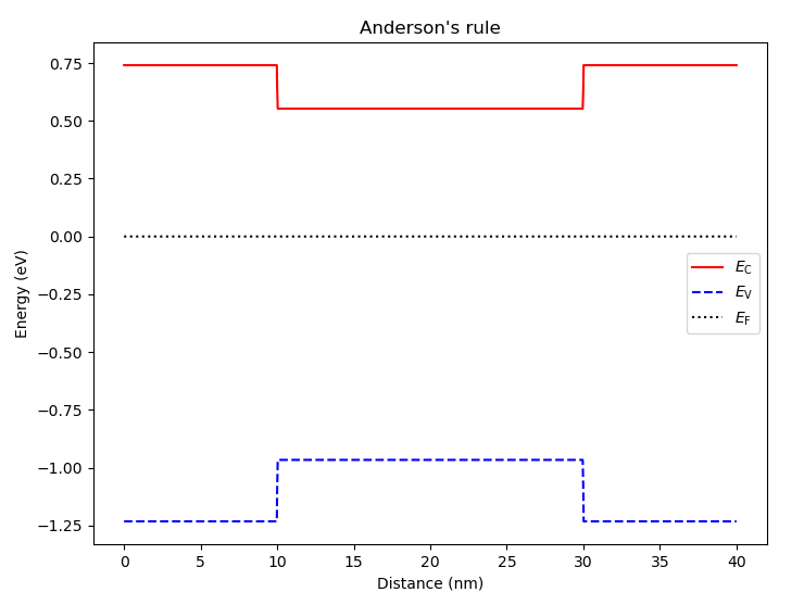
Fig. 6.4.1 Band alignment from Anderson’s rule
The total confinement potential \(V_\mathrm{conf}(x)\) for electrons will be set by the conduction band edge \(E_C\); see (2.1) and (2.2).
We first visualize the default confinement potential.
# View the total confinement potential before calling set_V_from_phi
an.plot(mesh, dvc.get_Vconf()/ct.e, ylabel="$V_\\mathrm{conf}$ (eV)",
   title="Before setting V from phi")
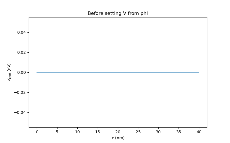
Fig. 6.4.2 Band alignment before setting the confinement potential
We see that, by default, there is no confinement potential in the device.
We then call
set_V_from_phi
to set the confinement potential to the conduction band edge.
# View the total confinement potential after calling set_V_from_phi
dvc.set_V_from_phi()
an.plot(mesh, dvc.get_Vconf()/ct.e, ylabel="$V_\\mathrm{conf}$ (eV)",
   title="After setting V from phi")
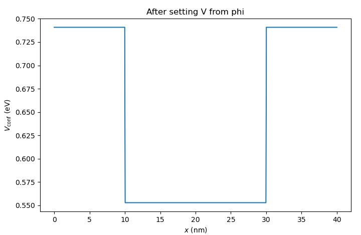
Fig. 6.4.3 Band alignment after setting the confinement potential
We see that this corresponds to the conduction band edge in Fig. 6.4.1.
6.4.5. Setting an external potential
We may set an external potential using the
set_Vext
method of the
Device
class. Here, we shift the barrier heights by \(0.5\textrm{ eV}\) upwards.
# Set an external potential to shift the barriers by +0.5 eV
dvc.set_Vext(0.5*ct.e, "left_barrier")
dvc.set_Vext(0.5*ct.e, "right_barrier")
an.plot(mesh, dvc.get_Vconf()/ct.e, ylabel="$V_\\mathrm{conf}$ (eV)",
   title="Shifted barrier heights")
This results in the following figure.
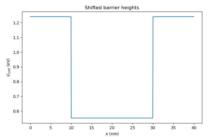
Fig. 6.4.4 Total confinement potential with barriers shifted upwards by \(0.5\ \mathrm{eV}\)
We may then remove the above external potential with
# Unset the external potential
dvc.set_Vext(0.0, "left_barrier")
dvc.set_Vext(0.0, "right_barrier")
6.4.6. Using band alignment parameters from RESCU
Band alignment parameters can be calculated from atomistic simulations (here,
performed using RESCU). The atomistic band alignment parameters for the
GaAs/AlGaAs heterojunction are stored in the
materials module, and may be activated by
calling the align_bands
method of the Device
class, with the GaAs material as the reference material (input argument). For
a theoretical background of this band alignment method, see
Band alignment from atomistic simulations.
# Use RESCU-fitted alignment parameters; choose GaAs as the reference layer
dvc.align_bands(mt.GaAs)
an.plot_bands(dvc, title="Band alignment from RESCU simulations")
This results in the following band diagram.
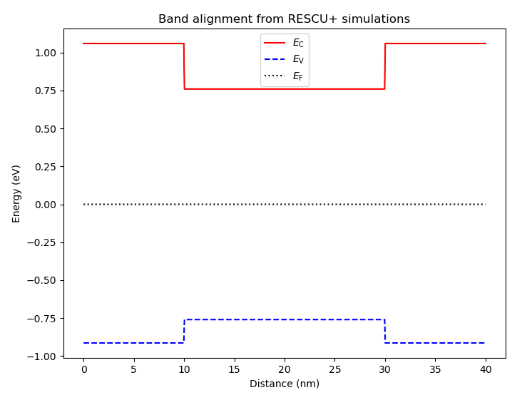
Fig. 6.4.5 Band diagram obtained using atomistic band alignment parameters evaluated with RESCU
We see that the band diagram is slightly different from the one obtained using Anderson’s rule, which is shown in Fig. 6.4.1.
6.4.7. Calculating and plotting envelope functions
To calculate envelope functions, we first set the confinement potential to correspond to the band diagram illustrated above. We then instantiate the Schrödinger solver on the device, solve Schrödinger’s equation, and print the resulting eigenenergies.
# Calculate the electron envelope functions
dvc.set_V_from_phi()
slv = Solver(dvc)
slv.solve()
dvc.print_energies()
The resulting energies are
Energy levels (eV)
[0.76997686 0.80131405 0.85313421 0.92433784 1.01099512 1.06706163
1.07137673 1.10643078 1.14911842 1.17786023]
while the minimum and maximum of the conduction band edge are \(0.76\textrm{ eV}\) and \(1.06\textrm{ eV}\), respectively. This means that five bound state can be obtained in this potential well. We inspect these states by plotting some of the envelope functions with
# Plot the first few levels
x = mesh.glob_nodes[:,0]
sort_indices = np.argsort(x)    # Sort the nodes along x
fig = plt.figure(figsize=(8,5))
ax = fig.add_subplot(1,1,1)
ax.set_xlabel("$x$ (nm)")
ax.set_ylabel("$\\psi(x)$")
ax.plot(x[sort_indices]/1e-9, dvc.eigenfunctions[sort_indices,0],
   "-k", label="Ground state")
ax.plot(x[sort_indices]/1e-9, dvc.eigenfunctions[sort_indices,1],
   "--b", label="1st excited state")
ax.plot(x[sort_indices]/1e-9, dvc.eigenfunctions[sort_indices,2],
   ":r", label="2nd excited state")
ax.legend()
plt.show()
This results in the following figure.
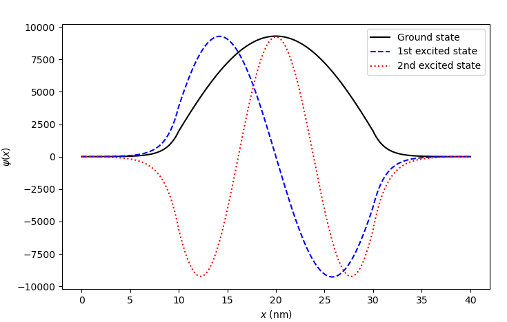
Fig. 6.4.6 Bound states in a potential well
We see that all these states look like the eigenstates of a rectangular potential well. By contrast with the eigenstates of an infinite potential well, these envelope functions penetrate slightly into the barrier regions.
We may verify that a deeper potential well results in more bound states
by shifting the bands by \(0.5\textrm{ eV}\) downwards in the well region. This is done
by shifting the reference potential \(\varphi_F\) with the
add_to_ref_potential
method of the
Device
class. Shifting the bands and plotting the result with
# Shift the bands in the well downwards by 0.5 eV
dvc.add_to_ref_potential(-0.5, region="well")
an.plot_bands(dvc,
   title="Band alignment from RESCU simulations with -0.5 eV shift in well")
results in
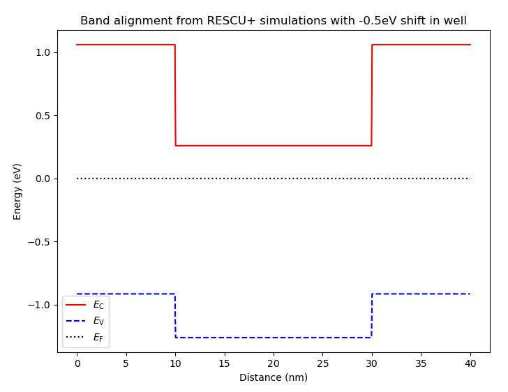
Fig. 6.4.7 Band diagram obtained using atomistic band alignment parameters evaluated with RESCU, with the potential well shifted by \(0.5\textrm{ eV}\) downwards
We can then update the confinement potential, instantiate a new Schrödinger solver, and solve again
# Update the confinement potential and solve Schrödinger again
dvc.set_V_from_phi()
slv = Solver(dvc)
slv.solve()
dvc.print_energies()
The resulting eigenenergies are then
Energy levels (eV)
[0.27117749 0.30618482 0.36443591 0.4457467  0.54975075 0.67569868
0.82186199 0.98254491 1.06856140 1.07127713]
We see that seven energy levels now lie between the conduction band minimum (\(0.26\textrm{ eV}\)) and maximum (\(1.06\textrm{ eV}\)).
Plotting the electron envelope functions, we see that we indeed have bound states which look essentially like those of the previous potential well.
# Plot the first few levels again
x = mesh.glob_nodes[:,0]
sort_indices = np.argsort(x)    # Sort the nodes along x
fig = plt.figure(figsize=(8,5))
ax = fig.add_subplot(1,1,1)
ax.set_xlabel("$x$ (nm)")
ax.set_ylabel("$\\psi(x)$")
ax.plot(x[sort_indices]/1e-9, dvc.eigenfunctions[sort_indices,0],
   "-k", label="Ground state")
ax.plot(x[sort_indices]/1e-9, dvc.eigenfunctions[sort_indices,1],
   "--b", label="1st excited state")
ax.plot(x[sort_indices]/1e-9, dvc.eigenfunctions[sort_indices,2],
   ":r", label="2nd excited state")
ax.legend()
plt.show()
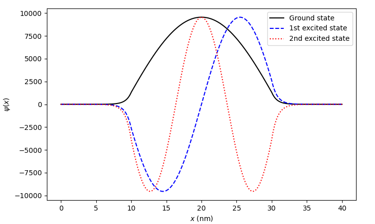
Fig. 6.4.8 Bound states in an artificially deeper potential well
6.5. Band alignment in SiGe/Si/SiGe and SiGe/Ge/SiGe heterostructures
Gate-defined quantum devices routinely employ epitaxial SiGe/Si/SiGe or SiGe/Ge/SiGe heterostructures to confine a two-dimensional carrier gas at an epitaxial interface [PB85, SKZ+21, Schaffler97, ZDM+13]. Two common examples are:
Electron qubits in tensile-strained Si wells: Electrons are confined within a Si layer grown on relaxed \(\text{Si}_{1-x}\text{Ge}_{x}\). The SiGe layer imposes a tensile strain on the Si layer, resulting in lifting of the six-fold degeneracy of the \(\Delta\) valley of Si. A conduction-band offset of \(\approx 0.18\ \mathrm{eV}\) at Ge concentration \(x\!\approx\!0.30\) is widely reported [SL92].
Hole qubits in compressively strained Ge wells: Holes are confined within a Ge layer grown on relaxed \(\text{Si}_{1-x}\text{Ge}_{x}\). The SiGe layer imposes a compressive strain on the Ge layer, resulting in selective confinement of holes and a valence-band offset of \(\approx 0.17\ \mathrm{eV}\) for \(x\!\approx\!0.75\) [TMW+21].
This section investigates band diagrams, band edge values, and confinement potentials for both systems using atomistic (RESCU) parameters.
6.5.1. Electron confinement in a SiGe/Si/SiGe heterostructure
We first define the materials of the heterostructure: relaxed
\(\text{Si}_{1-x}\text{Ge}_{x}\) (stored in mt.SiGe_DFT) and Si
strained on relaxed \(\text{Si}_{1-x}\text{Ge}_{x}\) (stored in
mt.Si_strained_on_SiGe).
# ----------------------------------------------
# Band alignment in SiGe/Si/SiGe heterostructure
# ----------------------------------------------

# materials for SiGe/Si/SiGe heterostructure
mt.SiGe_DFT.set_alloy_composition(0.30) # relaxed Si0.70Ge0.30 barriers
mt.Si_strained_on_SiGe.set_alloy_composition(0.30)
We may then define the device for this heterostructure.
# Create the device
dvc = Device(mesh, conf_carriers="e")
dvc.new_region("left_barrier", mt.SiGe_DFT)
dvc.new_region("well", mt.Si_strained_on_SiGe)
dvc.new_region("right_barrier", mt.SiGe_DFT)
The band alignment is then set using atomistic (RESCU) parameters.
# Align bands using the relaxed SiGe as the reference layer
dvc.align_bands(mt.SiGe_DFT)
The band diagram may then be plotted.
an.plot_bands(dvc, title="Si/SiGe band alignment (RESCU)")
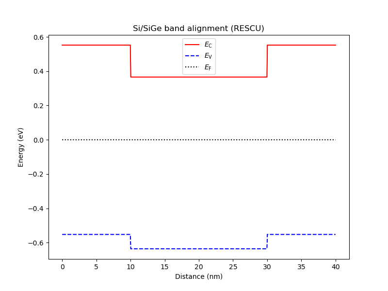
Fig. 6.5.1 Band diagram after RESCU band alignment. The conduction-band minimum and valence-band maximum are lower in the Si well than in the SiGe barrier. This type of band alignement is categorized as type-II band alignment.
The conduction-band and valence-band offsets (the variables cbo and vbo
below) are evaluated as the range (difference between the maximum and minimum
value, obtained via np.ptp) of unique (obtained via np.unique)
band-edge values across the device (stored in the variables cb and vb);
rounding (obtained via np.round) suppresses grid-level numerical noise.
# Conduction-band and valence-band offsets
cb  = dvc.cond_band_edge()/ct.e
cbo = np.ptp(np.unique(np.round(cb, 6)))
vb  = dvc.vlnce_band_edge()/ct.e
vbo = np.ptp(np.unique(np.round(vb, 6)))
print(f"SiGe/Si/SiGe heterostructure: VBO = {vbo:.6f} eV | CBO = {cbo:.6f} eV")
This results in the following values.
SiGe/Si/SiGe heterostructure: VBO = 0.057937 eV | CBO = 0.169713 eV
The confinement potential may also be plotted.
dvc.set_V_from_phi()
an.plot(mesh, dvc.get_Vconf()/ct.e, ylabel="$V_{\\mathrm{conf}}$ (eV)",
   title="Confinement potential (electron well)")
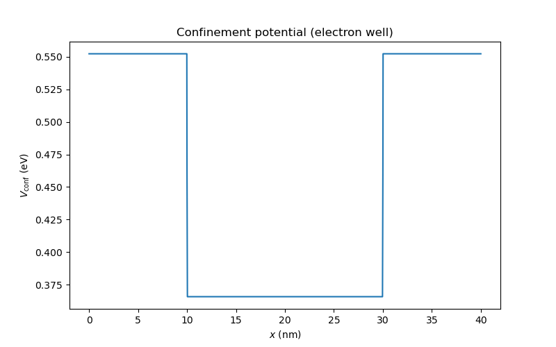
Fig. 6.5.2 Confinement potential extracted from the conduction band edge
6.6. Hole confinement in a SiGe/Ge/SiGe heterostructure
We first define the materials of the heterostructure in a way similar as for
the SiGe/Si/SiGe heterostructure. This time, we consider Ge strained on
relaxed \(\text{Si}_{1-x}\text{Ge}_{x}\) (stored in
mt.Ge_strained_on_SiGe).
# ----------------------------------------------
# Band alignment in SiGe/Ge/SiGe heterostructure
# ----------------------------------------------

# materials for SiGe/Ge/SiGe heterostructure
mt.SiGe_DFT.set_alloy_composition(0.75) # relaxed Si0.25Ge0.75 barriers
mt.Ge_strained_on_SiGe.set_alloy_composition(0.75)
The device for this heterostructure is created similarly as the previous one, with the exception that we set holes as the confined carriers.
# Create the device
dvc = Device(mesh, conf_carriers="h", hole_kp_model="luttinger_kohn_foreman")
dvc.new_region("left_barrier", mt.SiGe_DFT)
dvc.new_region("well", mt.Ge_strained_on_SiGe)
dvc.new_region("right_barrier", mt.SiGe_DFT)
dvc.align_bands(mt.SiGe_DFT)
The band diagram may then be plotted.
an.plot_bands(dvc, title="Ge/SiGe band alignment (RESCU)")
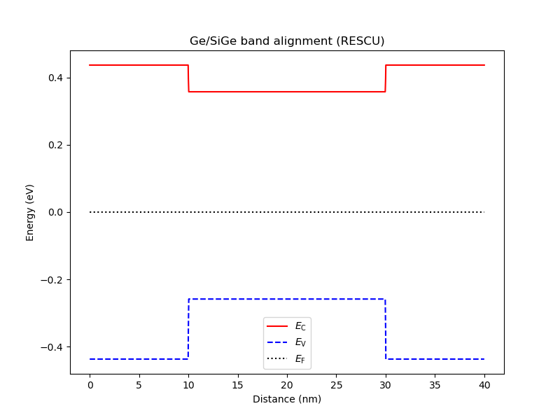
Fig. 6.6.1 Band diagram after RESCU band alignment. The valence-band maximum is higher in the Ge layer relative to the SiGe layers while the the conduction-band minimum is lower in the Ge layer relative to the SiGe layers. This is consistent with the type-I band alignments widely reported for planar Ge/SiGe at high Ge content [SKZ+21].
The conduction-band and valence-band offsets are evaluated as before.
vb  = dvc.vlnce_band_edge()/ct.e
vbo = np.ptp(np.unique(np.round(vb, 6)))
cb  = dvc.cond_band_edge()/ct.e
cbo = np.ptp(np.unique(np.round(cb, 6)))
print(f"SiGe/Ge/SiGe heterostructure: VBO = {vbo:.6f} eV | CBO = {cbo:.6f} eV")
This results in the following values.
SiGe/Ge/SiGe heterostructure: VBO = 0.176095 eV | CBO = 0.142431 eV
The valence-band offset \(0.176095\ \mathrm{eV}\) agrees with the \(\approx 0.170\ \mathrm{eV}\) offset reported in Ref. [TMW+21] for this composition, within \(\sim 0.01\ \mathrm{eV}\).
Finally, the confinement potential may be plotted.
dvc.set_V_from_phi()
an.plot(mesh, dvc.get_Vconf()/ct.e, ylabel="$V_{\\mathrm{conf}}$ (eV)",
   title="Confinement potential (hole well)")
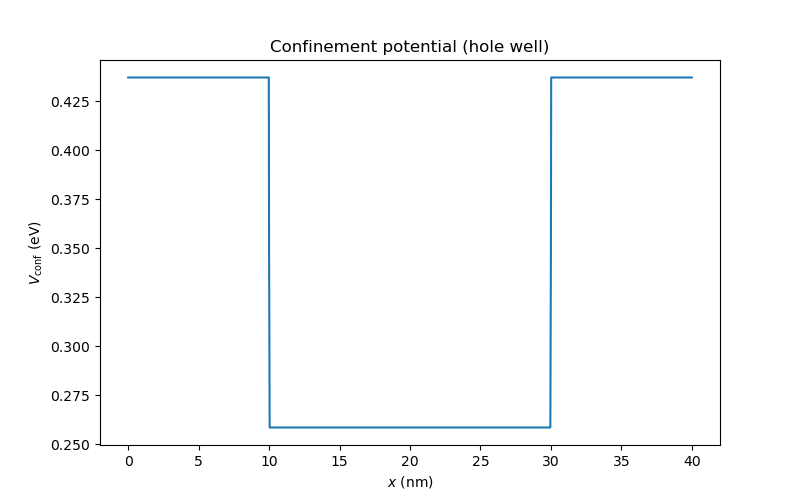
Fig. 6.6.2 Confinement potential extracted from the valence band edge
6.7. Offset sweep—Varying the Ge content in the SiGe substrates
Many designs tune the relaxed SiGe buffer composition \(x\) to optimize both strain and band offsets simultaneously. Here, we scan \(x \in [0,0.8]\) in seventeen steps and print the resulting band offsets for a SiGe/Si/SiGe heterostructure (electron well). We stop the sweep at \(x=0.8\). Indeed, for \(x>0.85\), the bandstructure of SiGe is Ge-like.
# -----------------------------------------------------------------------
# Offset sweep – varying Ge content in the SiGe substrates (SiGe/Si/SiGe)
# -----------------------------------------------------------------------
xs = np.linspace(0.0, 0.8, 17)
print("-"*31)
print("     x     VBO (eV)    CBO (eV)")
print("-"*31)

for xval in xs:
   # Composition-dependent materials
   mt.SiGe_DFT.set_alloy_composition(xval)
   mt.Si_strained_on_SiGe.set_alloy_composition(xval)

   # Device & alignment (electron well)
   dvc = Device(mesh, conf_carriers="e")
   dvc.new_region("left_barrier", mt.SiGe_DFT)
   dvc.new_region("well", mt.Si_strained_on_SiGe)
   dvc.new_region("right_barrier", mt.SiGe_DFT)
   dvc.align_bands(mt.SiGe_DFT)

   cb = dvc.cond_band_edge()/ct.e
   vb = dvc.vlnce_band_edge()/ct.e
   cbo = np.ptp(np.unique(np.round(cb, 6)))
   vbo = np.ptp(np.unique(np.round(vb, 6)))

   print(f"  {xval:0.3f}   {vbo:0.6f}    {cbo:0.6f}")
This results in the following data.
-------------------------------
   x     VBO (eV)    CBO (eV)
-------------------------------
0.000   0.000000    0.000000
0.050   0.009175    0.027031
0.100   0.018543    0.054562
0.150   0.028102    0.082598
0.200   0.037855    0.111133
0.250   0.047800    0.140172
0.300   0.057937    0.169713
0.350   0.068267    0.199754
0.400   0.078789    0.230298
0.450   0.089503    0.261345
0.500   0.100410    0.292893
0.550   0.111509    0.324942
0.600   0.122800    0.357495
0.650   0.134284    0.390549
0.700   0.145961    0.424104
0.750   0.157830    0.458162
0.800   0.169891    0.492722
Such tables are useful in several applications, such as when:
designing graded buffers to smoothly transition lattice constants;
stacking multiple wells with different barrier compositions;
optimizing tunnel rates in gate-defined quantum dots.
To adapt this sweep for a Ge well (SiGe/Ge/SiGe), replace the well material assignment from strained-Si to strained-Ge while keeping the SiGe reference.
6.8. Full code
__copyright__ = "Copyright 2022-2026, Nanoacademic Technologies Inc."

import numpy as np
from matplotlib import pyplot as plt
from pathlib import Path
from qtcad.device import constants as ct
from qtcad.device.mesh1d import Mesh
from qtcad.device import Device
from qtcad.device import materials as mt
from qtcad.device import analysis as an
from qtcad.device.schrodinger import Solver

# Path to mesh file
path = Path(__file__).parent.resolve()
path = path / "meshes" / "band_alignment.msh"

# Load the mesh
mesh = Mesh(1e-9, path)

# ----------------------------------------------------------------------
# GaAs/AlGaAs — Anderson’s rule, RESCU alignment, and Schrödinger solver
# ----------------------------------------------------------------------

# Create the device and add materials
dvc = Device(mesh, conf_carriers="e")

dvc.new_region("left_barrier", mt.AlGaAs)
dvc.new_region("well", mt.GaAs)
dvc.new_region("right_barrier", mt.AlGaAs)

# Show the band diagram obtained from Anderson's rule
an.plot_bands(dvc, title="Anderson's rule")

# View the total confinement potential before calling set_V_from_phi
an.plot(
    mesh,
    dvc.get_Vconf() / ct.e,
    ylabel="$V_\\mathrm{conf}$ (eV)",
    title="Before setting V from phi",
)

# View the total confinement potential after calling set_V_from_phi
dvc.set_V_from_phi()
an.plot(
    mesh,
    dvc.get_Vconf() / ct.e,
    ylabel="$V_\\mathrm{conf}$ (eV)",
    title="After setting V from phi",
)

# Set an external potential to shift the barriers by +0.5 eV
dvc.set_Vext(0.5 * ct.e, "left_barrier")
dvc.set_Vext(0.5 * ct.e, "right_barrier")
an.plot(
    mesh,
    dvc.get_Vconf() / ct.e,
    ylabel="$V_\\mathrm{conf}$ (eV)",
    title="Shifted barrier heights",
)

# Unset the external potential
dvc.set_Vext(0.0, "left_barrier")
dvc.set_Vext(0.0, "right_barrier")

# Use RESCU-fitted alignment parameters; choose GaAs as the reference layer
dvc.align_bands(mt.GaAs)
an.plot_bands(dvc, title="Band alignment from RESCU simulations")

# Calculate the electron envelope functions
dvc.set_V_from_phi()
slv = Solver(dvc)
slv.solve()
dvc.print_energies()

# Plot the first few levels
x = mesh.glob_nodes[:, 0]
sort_indices = np.argsort(x)  # Sort the nodes along x
fig = plt.figure(figsize=(8, 5))
ax = fig.add_subplot(1, 1, 1)
ax.set_xlabel("$x$ (nm)")
ax.set_ylabel("$\\psi(x)$")
ax.plot(
    x[sort_indices] / 1e-9,
    dvc.eigenfunctions[sort_indices, 0],
    "-k",
    label="Ground state",
)
ax.plot(
    x[sort_indices] / 1e-9,
    dvc.eigenfunctions[sort_indices, 1],
    "--b",
    label="1st excited state",
)
ax.plot(
    x[sort_indices] / 1e-9,
    dvc.eigenfunctions[sort_indices, 2],
    ":r",
    label="2nd excited state",
)
ax.legend()
plt.show()

# Shift the bands in the well downwards by 0.5 eV
dvc.add_to_ref_potential(-0.5, region="well")
an.plot_bands(
    dvc, title="Band alignment from RESCU simulations with -0.5 eV shift in well"
)

# Update the confinement potential and solve Schrödinger again
dvc.set_V_from_phi()
slv = Solver(dvc)
slv.solve()
dvc.print_energies()

# Plot the first few levels again
x = mesh.glob_nodes[:, 0]
sort_indices = np.argsort(x)  # Sort the nodes along x
fig = plt.figure(figsize=(8, 5))
ax = fig.add_subplot(1, 1, 1)
ax.set_xlabel("$x$ (nm)")
ax.set_ylabel("$\\psi(x)$")
ax.plot(
    x[sort_indices] / 1e-9,
    dvc.eigenfunctions[sort_indices, 0],
    "-k",
    label="Ground state",
)
ax.plot(
    x[sort_indices] / 1e-9,
    dvc.eigenfunctions[sort_indices, 1],
    "--b",
    label="1st excited state",
)
ax.plot(
    x[sort_indices] / 1e-9,
    dvc.eigenfunctions[sort_indices, 2],
    ":r",
    label="2nd excited state",
)
ax.legend()
plt.show()

# ----------------------------------------------
# Band alignment in SiGe/Si/SiGe heterostructure
# ----------------------------------------------

# materials for SiGe/Si/SiGe heterostructure
mt.SiGe_DFT.set_alloy_composition(0.30)  # relaxed Si0.70Ge0.30 barriers
mt.Si_strained_on_SiGe.set_alloy_composition(0.30)

# Create the device
dvc = Device(mesh, conf_carriers="e")
dvc.new_region("left_barrier", mt.SiGe_DFT)
dvc.new_region("well", mt.Si_strained_on_SiGe)
dvc.new_region("right_barrier", mt.SiGe_DFT)

# Align bands using the relaxed SiGe as the reference layer
dvc.align_bands(mt.SiGe_DFT)

an.plot_bands(dvc, title="Si/SiGe band alignment (RESCU)")

# Conduction-band and valence-band offsets
cb = dvc.cond_band_edge() / ct.e
cbo = np.ptp(np.unique(np.round(cb, 6)))
vb = dvc.vlnce_band_edge() / ct.e
vbo = np.ptp(np.unique(np.round(vb, 6)))
print(f"SiGe/Si/SiGe heterostructure: VBO = {vbo:.6f} eV | CBO = {cbo:.6f} eV")

dvc.set_V_from_phi()
an.plot(
    mesh,
    dvc.get_Vconf() / ct.e,
    ylabel="$V_{\\mathrm{conf}}$ (eV)",
    title="Confinement potential (electron well)",
)

# ----------------------------------------------
# Band alignment in SiGe/Ge/SiGe heterostructure
# ----------------------------------------------

# materials for SiGe/Ge/SiGe heterostructure
mt.SiGe_DFT.set_alloy_composition(0.75)  # relaxed Si0.25Ge0.75 barriers
mt.Ge_strained_on_SiGe.set_alloy_composition(0.75)

# Create the device
dvc = Device(mesh, conf_carriers="h", hole_kp_model="luttinger_kohn_foreman")
dvc.new_region("left_barrier", mt.SiGe_DFT)
dvc.new_region("well", mt.Ge_strained_on_SiGe)
dvc.new_region("right_barrier", mt.SiGe_DFT)
dvc.align_bands(mt.SiGe_DFT)

an.plot_bands(dvc, title="Ge/SiGe band alignment (RESCU)")

vb = dvc.vlnce_band_edge() / ct.e
vbo = np.ptp(np.unique(np.round(vb, 6)))
cb = dvc.cond_band_edge() / ct.e
cbo = np.ptp(np.unique(np.round(cb, 6)))
print(f"SiGe/Ge/SiGe heterostructure: VBO = {vbo:.6f} eV | CBO = {cbo:.6f} eV")

dvc.set_V_from_phi()
an.plot(
    mesh,
    dvc.get_Vconf() / ct.e,
    ylabel="$V_{\\mathrm{conf}}$ (eV)",
    title="Confinement potential (hole well)",
)

# -----------------------------------------------------------------------
# Offset sweep – varying Ge content in the SiGe substrates (SiGe/Si/SiGe)
# -----------------------------------------------------------------------
xs = np.linspace(0.0, 0.8, 17)
print("-" * 31)
print("     x     VBO (eV)    CBO (eV)")
print("-" * 31)

for xval in xs:
    # Composition-dependent materials
    mt.SiGe_DFT.set_alloy_composition(xval)
    mt.Si_strained_on_SiGe.set_alloy_composition(xval)

    # Device & alignment (electron well)
    dvc = Device(mesh, conf_carriers="e")
    dvc.new_region("left_barrier", mt.SiGe_DFT)
    dvc.new_region("well", mt.Si_strained_on_SiGe)
    dvc.new_region("right_barrier", mt.SiGe_DFT)
    dvc.align_bands(mt.SiGe_DFT)

    cb = dvc.cond_band_edge() / ct.e
    vb = dvc.vlnce_band_edge() / ct.e
    cbo = np.ptp(np.unique(np.round(cb, 6)))
    vbo = np.ptp(np.unique(np.round(vb, 6)))

    print(f"  {xval:0.3f}   {vbo:0.6f}    {cbo:0.6f}")