7. Visualizing QTCAD quantities with ParaView

7.1. Requirements

7.1.1. Software components

• ParaView

7.1.2. References

• Schrödinger equation for a quantum dot

7.2. Briefing

The goal of this tutorial is to demonstrate how to visualize certain quantities generated by QTCAD using ParaView. The quantities we will be visualizing are those simulated in creating_dot.py (see Schrödinger equation for a quantum dot for details).

7.3. Opening ParaView

The first step to visualizing the QTCAD quantities is to open ParaView. Clicking on the icon should lead you to the following GUI.

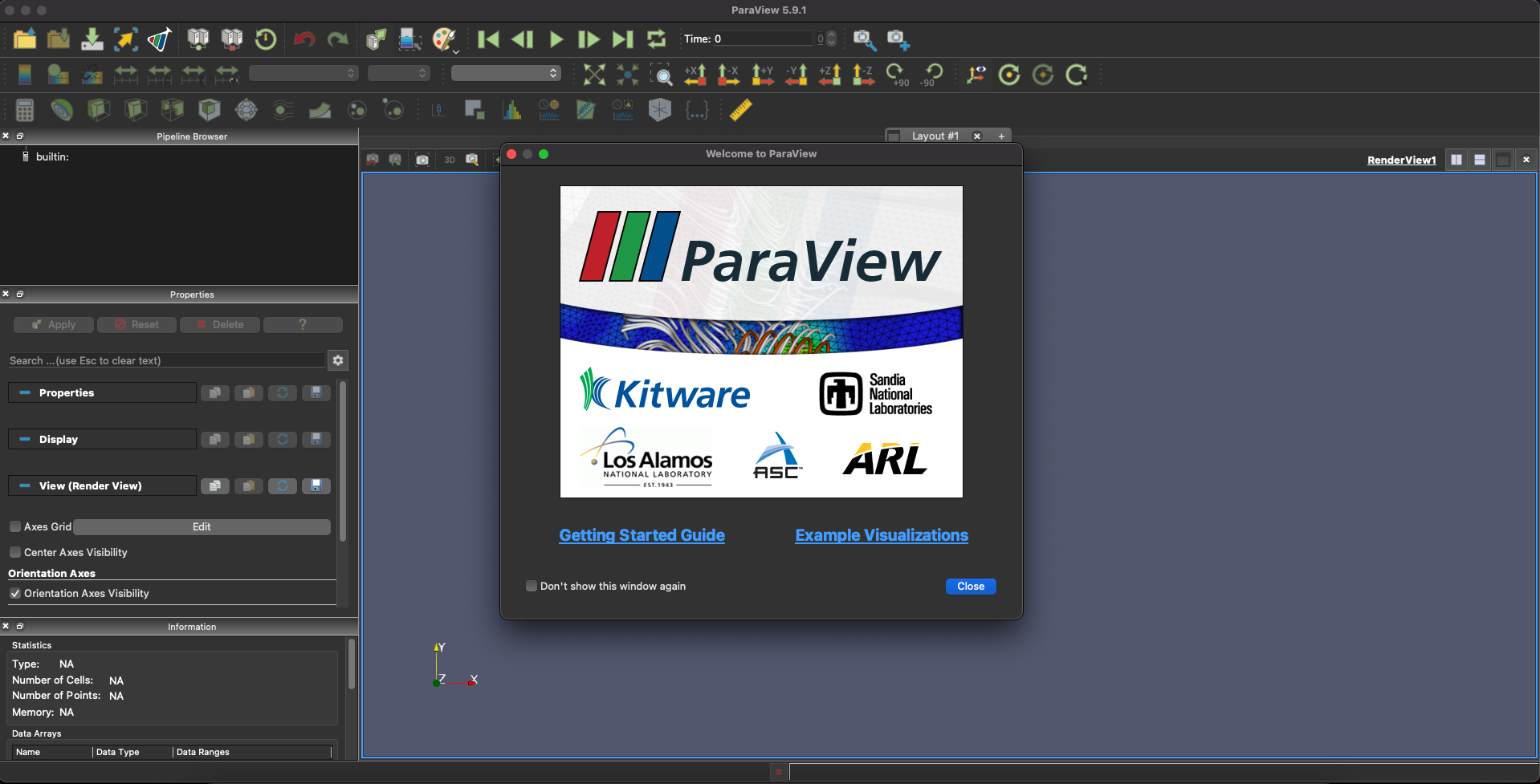
Fig. 7.3.1 ParaView’s startup page

We close the popup and are ready to begin.

7.4. Visualizing the potential

We start by looking at the conduction band edge. We use the file>open menu to select the file containing the conduction band edge in .vtu format.

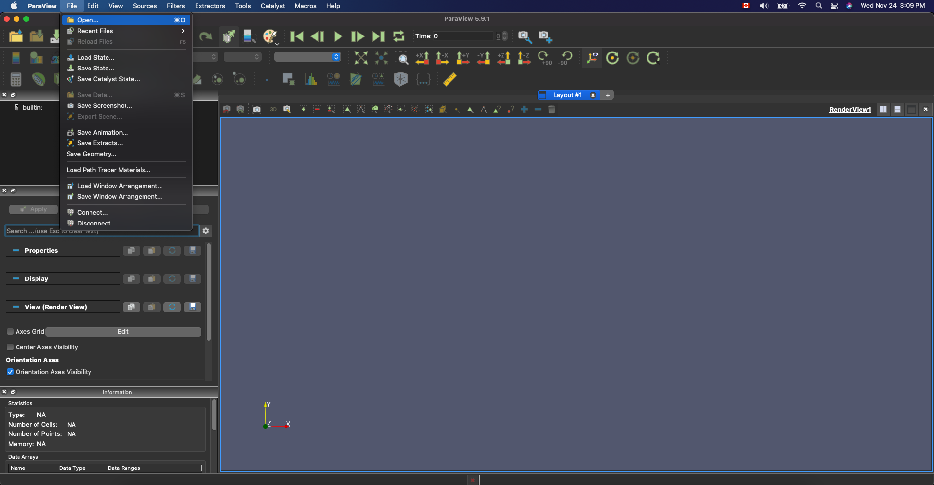
Fig. 7.4.1 From top menu we click on open and find the desired file.

What should appear is a color plot of the potential applied to the system.

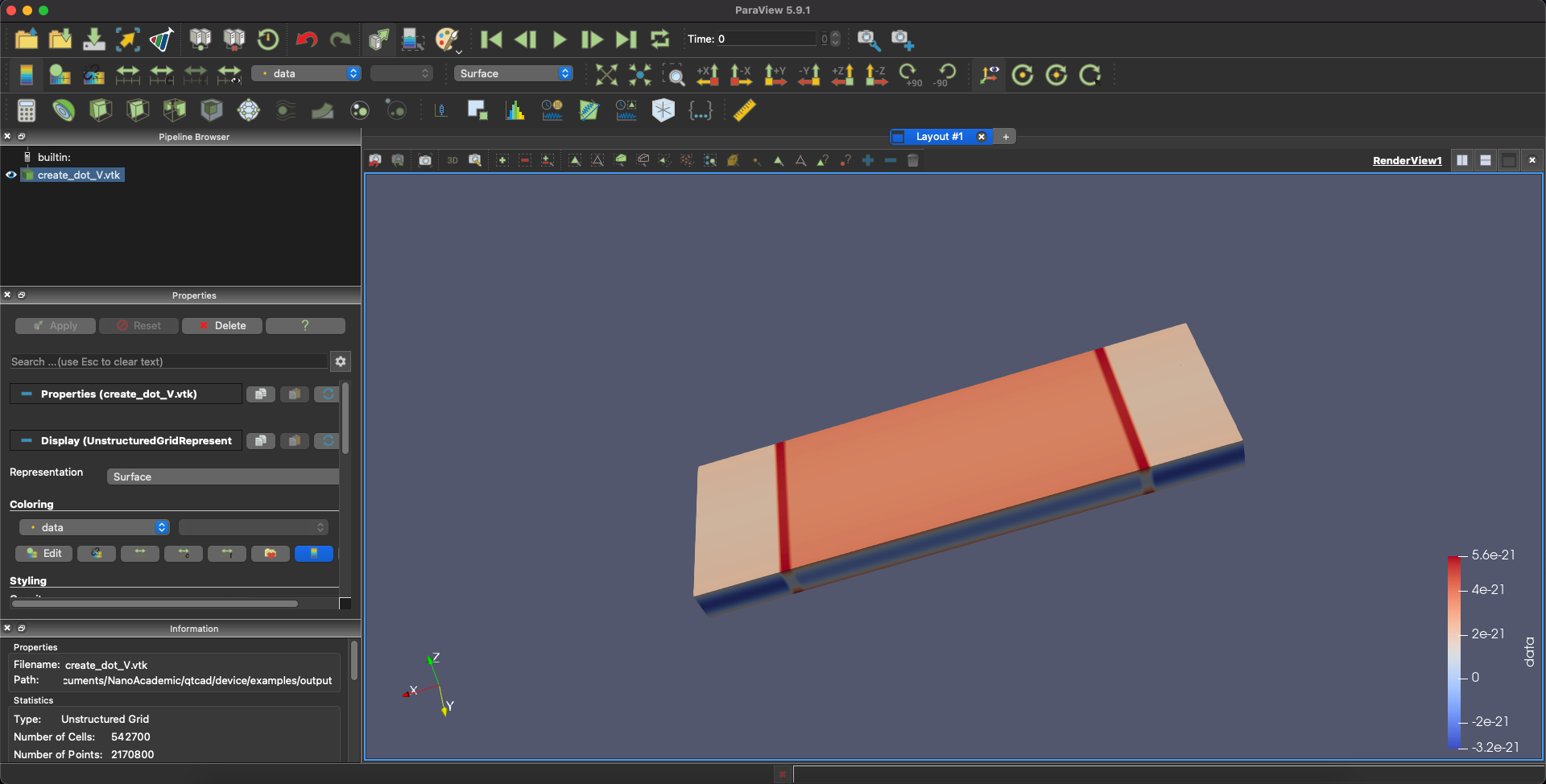
Fig. 7.4.2 Confinement potential over the device.

We see that along the \(x\) direction, the potential has 2 barriers in dark red. We should also be able to make out the parabolic nature of the potential along the \(y\) and \(z\) directions.

Before moving on to visualizing the wavefunctions, we will delete the conduction band edge plot using the delete button on the left.

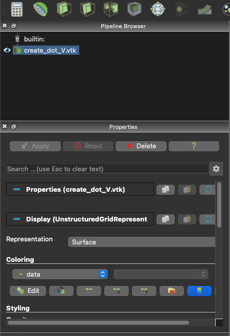
Fig. 7.4.3 In the left interface of ParaView we can delete or hide loaded files.

7.5. Visualizing wavefunctions

Next we visualize the wavefunctions. We start by opening the .vtu file containing the ground state.

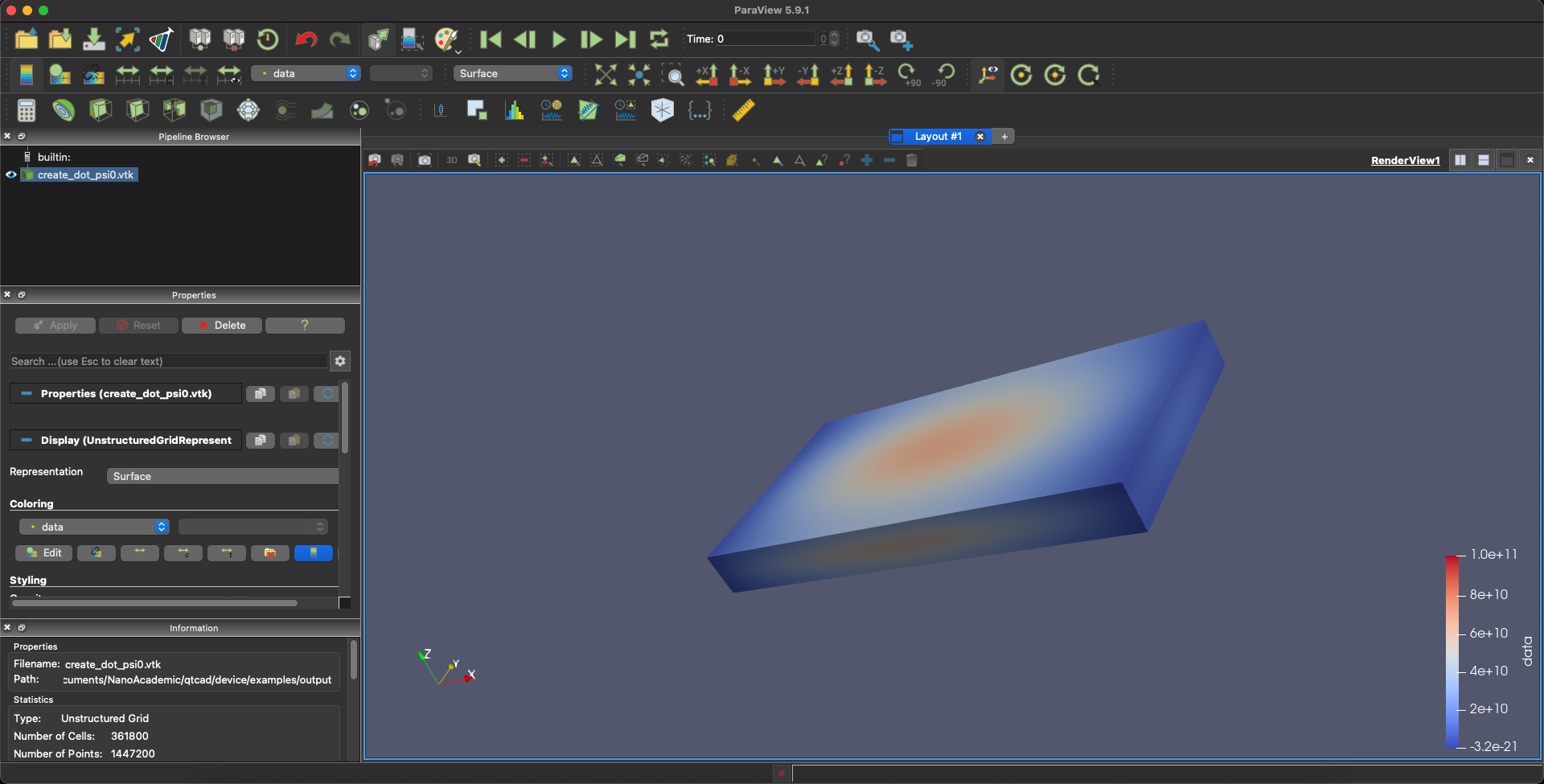
Fig. 7.5.1 Visualization of the ground state in ParaView.

What we see when the file opens is the value of the wavefunction on the outer boundary of the dotmesh. To see the wavefunction inside this region, we use the clip tool which is the third tool on the menu bar.

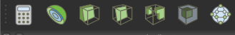
Fig. 7.5.2 clip tools

Once selected, we can choose where the structure will be clipped by modifying the origin in the plane parameters on the right-hand side.

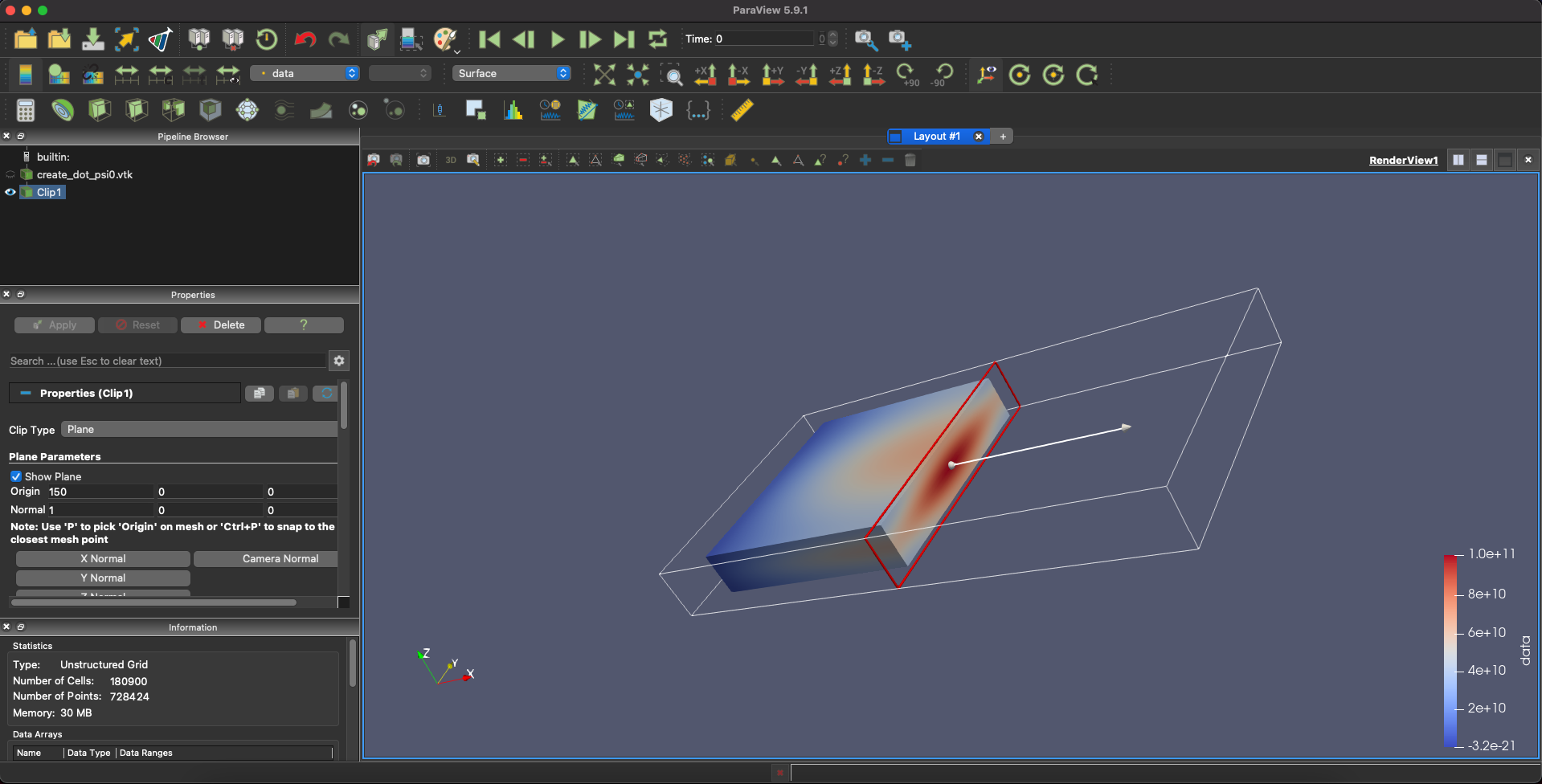
Fig. 7.5.3 Clipped the device perpendicular to the x-direction.

We can also use the plane parameters to define the normal vector of the clip, e.g. along the \(z\) direction in this example.

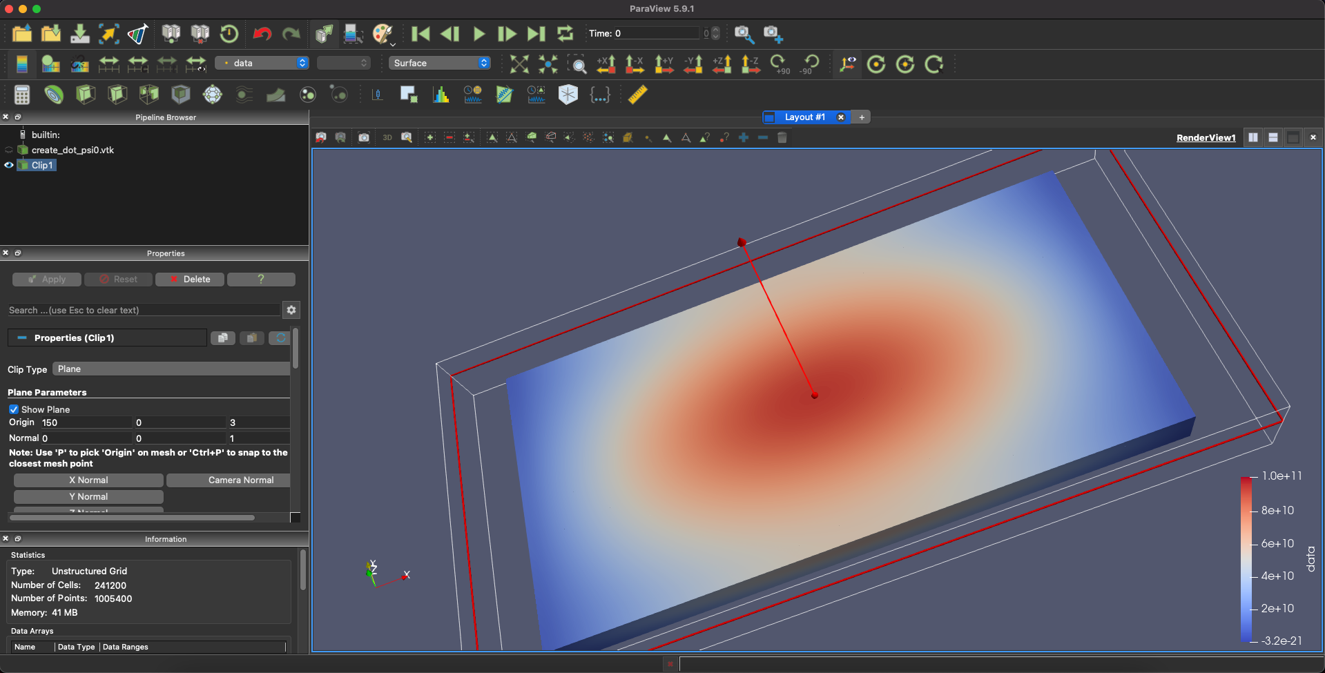
Fig. 7.5.4 Clipped the device perpendicular to the z-direction.

From these clips, we can see that the electron is concentrated at the center of this structure.

Then, in the top right corner, we can choose to split the screen from left to right.

Fig. 7.5.5 We can split the screen to obtain two interfaces using the button in the top right menu.

We will then see an empty ParaView window on the right.

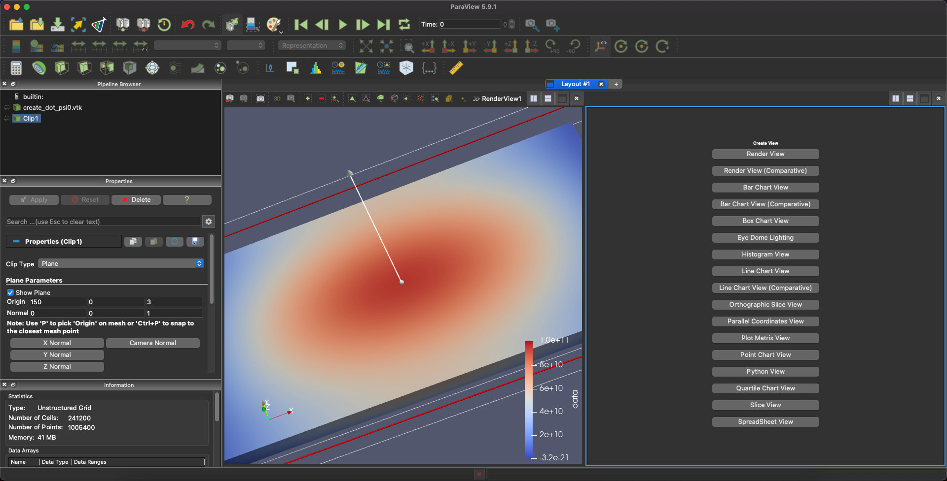
Fig. 7.5.6 ParaView interface with two screens.

From there, we can open the first excited state in this second view window.

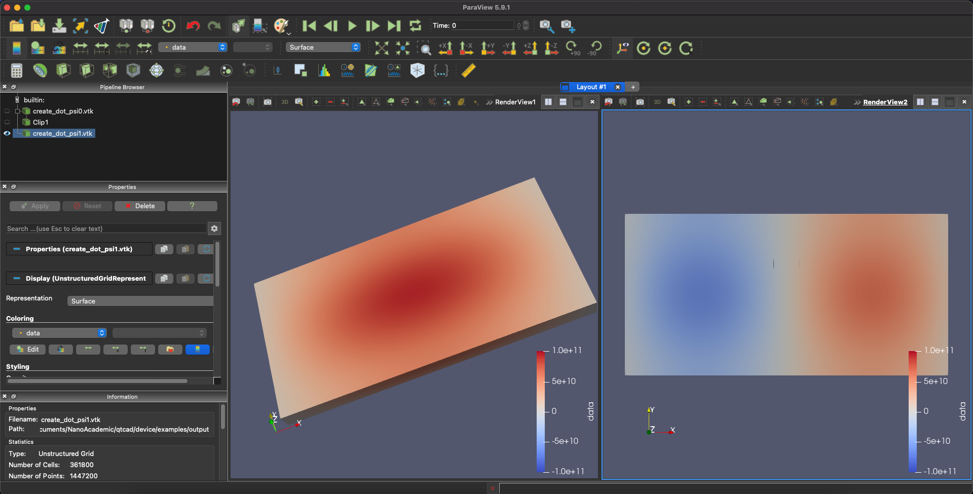
Fig. 7.5.7 ParaView interface with both ground state and first excited state visualized.

From here, we can also take linecuts using the plot over line tool.

Fig. 7.5.8 Linecut button located on the third row in the top menu.

The two points used to define the line can be specified on the right under the line parameters heading. The line can also be seen in the view window.

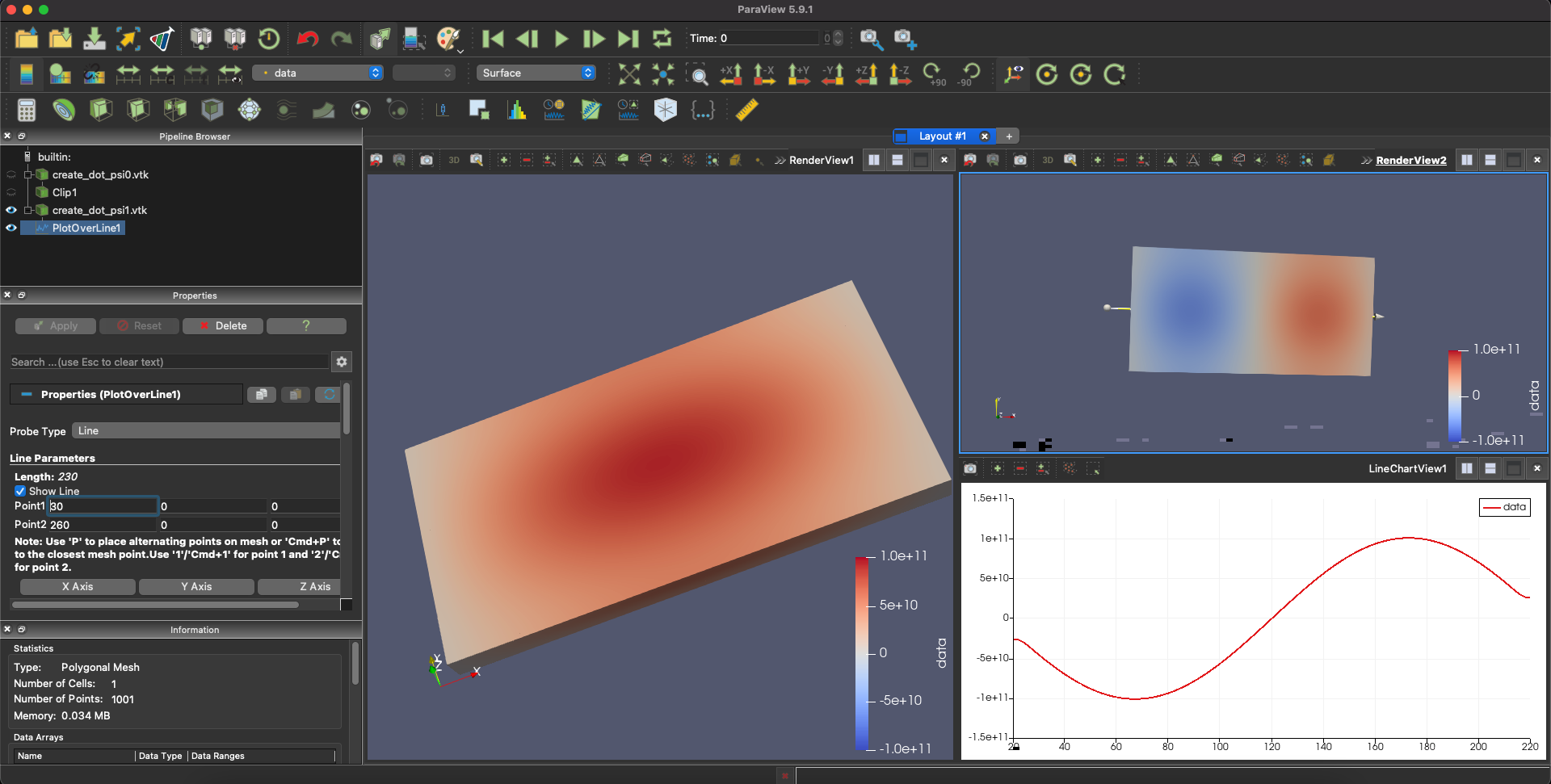
Fig. 7.5.9 Line plot

The resulting line plot along x shows the sinusoidal wavefunction we expect for a particle-in-a box potential.

7.6. Visualizing datasets

Next we show how to visualize any simulated data over various regions. If we use the .vtu format any information about regions of the mesh won’t be stored. However, by using the .vtm format, we can choose to show only specific regions and visualize any simulated data within those selected areas. We start by opening the .vtm file. Please make sure there’s a folder with the same name as the file in the same location. This is required for it to work properly.

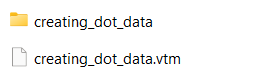
Fig. 7.6.1 a .vtm file should have a folder with the same name.

As we successfully load the .vtm file in ParaView. We should have a similar interface as loading a .vtu file.

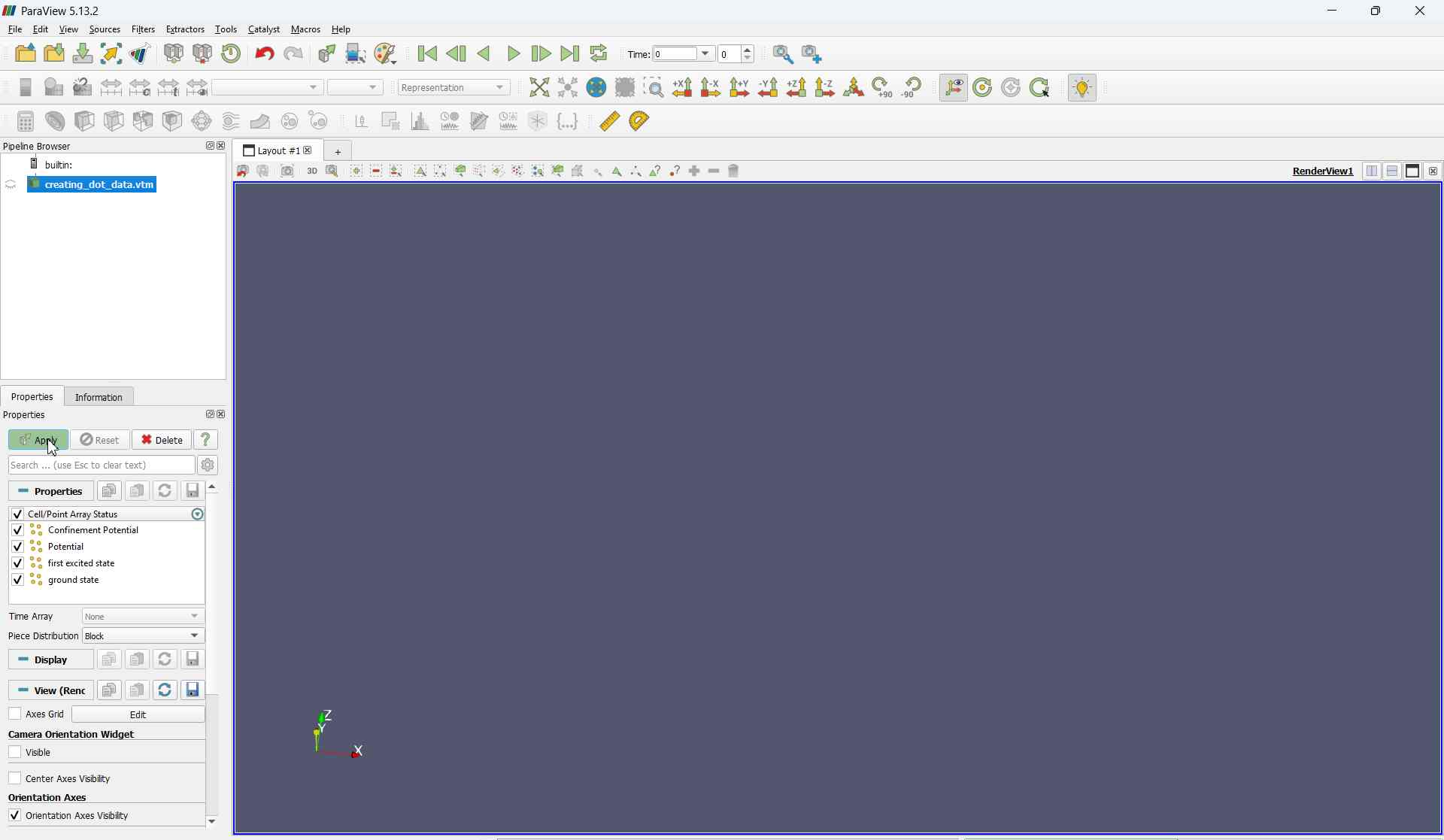
Fig. 7.6.2 ParaView interface after successfully loading the .vtm file.

Next we navigatie through the menu and select the MultiBlock Inspector from View>MultiBlock Inspector.

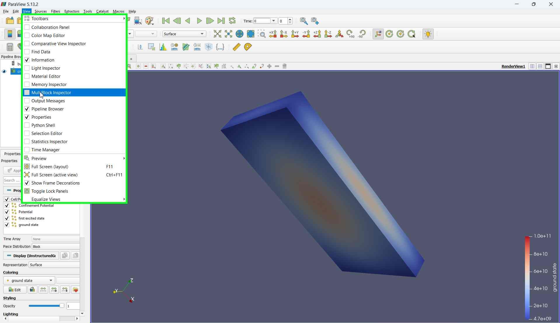
Fig. 7.6.3 Selecting MultiBlock Inspector from View

A new interface should pop up on the right side. From there, we can see the region names stored in the mesh and toggle them on or off to hide or select them as needed.

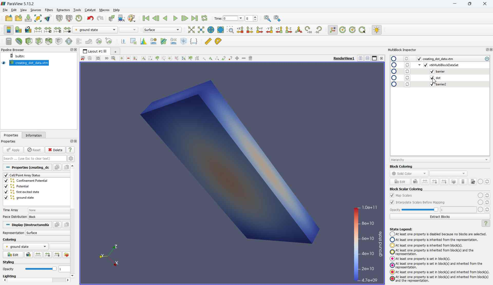
Fig. 7.6.4 We can toggle various regions in the new interface on the right to hide them.

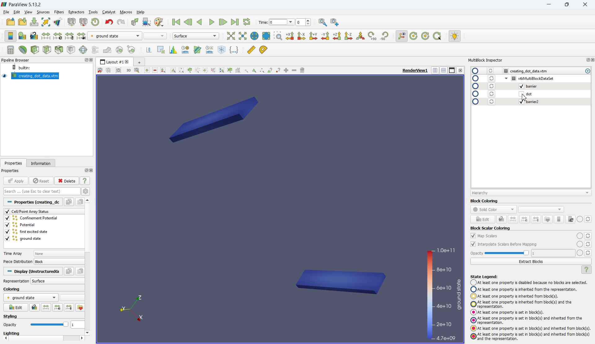
Fig. 7.6.5 Hiding the dot region as an example.

7.7. Conclusion

Presented above are the main tools we use in ParaView to analyze outputs of QTCAD. However, ParaView is very flexible. There are therefore most likely other tools that may also be useful.