10. Including spin–orbit coupling and magnetic effects in a simulation
10.1. Requirements
10.1.1. Software components
QTCAD
Gmsh
10.1.2. Geometry file
qtcad/examples/tutorials/meshes/box.geo
10.1.3. Python script
qtcad/examples/tutorials/holes_soc_B.py
10.1.4. References
10.2. Briefing
In this tutorial, we explain how to include spin–orbit coupling and magnetic effects (both Zeeman and orbital effects) in a QTCAD simulation. We will investigate how spin–orbit coupling can modify the spectrum of a hole in a box.
The full code may be found at the bottom of this page,
or in qtcad/examples/tutorials/hole_soc_B.py.
10.3. Setting up the device
10.3.1. Header
Like most python scripts, we start with a header. The header is used to import the relevant modules that will be used in this example.
import numpy as np
from matplotlib import pyplot as plt
import matplotlib.lines as mlines
from progress.bar import ChargingBar as Bar
import pathlib

from qtcad.device import materials as mt
from qtcad.device import constants as ct
from qtcad.device.pauli import J_x, J_y

from qtcad.device import Device
from qtcad.device.schrodinger import Solver, SolverParams
from qtcad.device.mesh3d import Mesh
The first group of imports are from standard python libraries.
The second group contains constants and material properties.
While the materials and
constants modules have been described in
previous tutorial, the pauli module is introduced
here.
This module contains the Pauli matrices for both spin-\(1/2\) and
spin-\(3/2\) particles.
Here, we have imported J_x and J_y which are the \(x\) and \(y\)
spin-\(3/2\) Pauli matrices.
The third group of imports contains modules that allow us to create the
mesh, the
device,
and solve the Schrödinger equation.
10.3.2. Setup
After importing the relevant modules, we set up our calculation.
This step involves defining constants and creating the
mesh and the
device over which the simulation will be
run.
#-------------------------------------------------------------------------------
# Setup
#-------------------------------------------------------------------------------
# Constants
nm = 1e-9
A = 1e-10
meV = ct.e/1000
Here we define three constants: nm, A, and meV which define
nanometers, Angstroms, and millielectronvolts in SI units.
Next we set up paths to input and output files
# Names of files ---------------------------------------------------------------
path = pathlib.Path(__file__).parent.resolve()

# Output
n_no_soc = "hole_energies_vs_B"
n_soc = "hole_energies_withSOC_vs_B"
n_kz2 = "kz2_holes"
n_plot = "holes_energies_vs_B"

# Input
n_mesh = "box.msh"
The first line defines the path to the script being run.
We then define the names to certain output data files and the name of the mesh
file that we will load.
After the preliminary constants have been defined, we create a
Mesh object
# Initialize the meshes --------------------------------------------------------
path_mesh = str(path/"meshes"/f"{n_mesh}")
# Load the mesh
scaling = nm
mesh = Mesh(scaling, path_mesh)
from which we then create a Device object
# Create device ------------------------------------------------------------
# Create device from mesh
d = Device(mesh, conf_carriers="h", hole_kp_model = "luttinger_kohn_foreman")

# Create regions
d.new_region("domain", mt.GaAs)

# Then create insulator boundaries
d.new_insulator("bnd")
The system we have created is a box made of GaAs with dimensions
\(60\mathrm{nm} \times 60\mathrm{nm} \times 3\mathrm{nm}\).
The device, d, is defined over this box and will contain holes as confined
carriers, which we model using the 4-band "luttinger_kohn_foreman" model.
We have also enforced “insulator” boundary conditions at the edges of the box
which will indicate to the Schrödinger
Solver that the
wavefunctions should vanish at the boundaries of the box.
10.4. Solving the Schrödinger equation with a magnetic field
Now that the Device, d has been
initialized, we can solve the Schrödinger equation.
We start by setting up the Schrödinger
SolverParams.
#-------------------------------------------------------------------------------
# Solving Schrodinger Equation with a magnetic field
#-------------------------------------------------------------------------------
print("-------------------------------------------------------")
print("Solving Schrodinger Equation including B field")
print("-------------------------------------------------------")
# Set up solver parameters -------------------------------------------------
# Configure and create the Schrodinger solver
params_schrod = SolverParams()
params_schrod.num_states = 10
params_schrod.verbose = False
Then we add a magnetic field, \(\mathbf B = B_0 \hat{z}\), to the system. We will solve the Schrödinger equation for different magnetic field strengths, \(B_0\), from \(0\mathrm{T}\) to \(10\mathrm{T}\).
# Set up B field ---------------------------------------------------------------
B = 10
B_vec = np.linspace(0, 1, 6) * B
# use a progress bar
progress_bar = Bar("B loop", max = len(B_vec))
In the above snippet we have also set up a progress bar, Bar, to track the
calculation.
Next, we loop over the applied magnetic fields.
For each given field, we use the
set_Bfield method to set the
field over the Device, d.
This method takes as input the applied magnetic field, np.array([0, 0, B]),
in this case, and the gauge to be used when including the orbital magnetic
effects.
Here, we use the "landau" gauge.
Another possible option would be the "symmetric" gauge.
By setting the magnetic field for the device, we automatically include both the
Zeeman and orbital magnetic effects in the calculation.
data = np.zeros((len(B_vec), params_schrod.num_states + 1))

for i, B0 in enumerate(B_vec):
   # include B in the calculation
   d.set_Bfield(np.array([0, 0, B0]), gauge="landau")

   # Solve --------------------------------------------------------------------
   # Create Schrodinger solver
   ss = Solver(d, solver_params=params_schrod)
   ss.solve()

   # Print results
   print("\n-----------------------------")
   print(f"B = {B0}")
   d.print_energies()
   # Update progress bar
   progress_bar.next()
   print("\n-----------------------------\n")

   # Save results to file
   data[i, 0] = B0
   data[i, 1:] = d.energies/ct.e
   with open(str( path / "output" / f"{n_no_soc}.txt" ), "w") as f:
      np.savetxt(f, data)
After setting the magnetic filed, we create a Schrödinger
Solver and
solve the Schrödinger equation.
We then write the energies to a file.
We emphasize that these energies will be the particle-in-a box energies for a
hole under the 4-band "luttinger_kohn_foreman" model subject to a constant
magnetic field along \(z\) (including both Zeeman and orbital magnetic
effects).
After the loop is complete, the energies for different magnetic field strengths
are saved to "data/hole_energies_withSOC_vs_B.txt".
Note
The QTCAD convention for the hole eigenenergies is one where both the effective mass and charge are positive and the states are labeled with the quantum numbers of missing electrons (see QTCAD convention for holes for more details).
Note
The set_Bfield method can
also be used to include a position-dependent magnetic field.
In this case the first input of
set_Bfield will be a 2D array
and will contain the magnetic field at every global node of the device.
However, when the magnetic field is not constant, orbital magnetic effects
cannot be included in the model and are turned off by default.
Note
It is possible to turn on/off the orbital and/or Zeeman effects even when
a magnetic field is applied using the
set_Zeeman and
set_orb_B_effects
setters respectively.
10.5. Including spin–orbit coupling
Now, we will include spin–orbit coupling in the same calculations and compare to see how the energies change. This comparison will give us an idea of the importance of spin–orbit coupling in this type of system. The specific type of spin–orbit coupling we consider is of the form
where we denote half of the anticommutator as \(\{A, B\} = (AB + BA) / 2\), \(\beta\) is the strength of the spin–orbit coupling, and \(\mathbf J\) is the vector of spin-3/2 matrices
As explained in Cubic spin-orbit couplings, we can approximate the cubic spin–orbit coupling of Eq. (10.5.1) with a linear version
To implement the linear version, we need to compute \(\left<k_z^2\right>\).
For the approximation to hold, all the eigenstates should have the same value
of \(\left<k_z^2\right>\).
Using the get_k_squared
method, we compute the \(\left<k_z^2\right>\) for all the eigenstates and
then store the values in a file "data/kz2_holes.txt".
#-------------------------------------------------------------------------------
# Solving Schrodinger Equation with a magnetic field and SOC
#-------------------------------------------------------------------------------
print("-------------------------------------------------------")
print("Solving Schrodinger Equation including B field and SOC")
print("-------------------------------------------------------")

# Set up SOC -------------------------------------------------------------------
# Compute <k_z^2>
kz2 = np.array([d.get_k_squared(i) for i in range(params_schrod.num_states)])

with open(str( path / "output" / f"{n_kz2}.txt" ), "w") as f:
   np.savetxt(f, kz2)
The get_k_squared method has
two keyword arguments.
The first tells it which state we wish to compute \(\left<k_j^2\right>\)
for (defaults to \(0\), i.e. the ground state) and the second gives the
values of \(j\).
By default, \(j=2\) which implies \(\left<k_z^2\right>\) (\(j=0\)
implies \(\left<k_x^2\right>\) and \(j=1\) implies
\(\left<k_y^2\right>\)).
Note
Using the get_k_squared
method at this point of the script will compute \(\left<k_z^2\right>\)
for the states stored in the
eigenfunctions
attribute of the Device, d.
These states are those subject to a magnetic field \(B_0=10\mathrm{T}\).
We expect \(\left<k_z^2\right>\) to be independent of \(B_0\)
because the magnetic field is out of plane and should therefore only affect
the in-plane confinement.
Consequently, the values in kz2 can be used for any value of
\(B_0\).
We add the linear version of the spin–orbit coupling [Eq.
(10.5.2)] to the device using the
set_soc method
# Coupling coefficient
beta = 82 * ct.e * A**3
# Add SOC to the device
d.set_soc([beta * kz2[0] * J_x, -beta * kz2[0] * J_y, None])
The argument of the set_soc method
is a list with 3 entries.
Each entry represents the coupling to \(k_x\), \(k_y\), and \(k_z\)
respectively.
Moreover, the entries should be 2D square arrays with dimension equal to the
number of bands in the model.
For electrons, the arrays are \(2 \times 2\) because the indices run over
the spin of the electron.
In this case, for holes in the 4-band Luttinger-Kohn-Foreman model, they are
\(4 \times 4\).
When an entry is None the coupling for the associated \(k\) direction
is neglected [\(k_x\) associated to the first entry (0 in python indexing),
\(k_y\) associated to the second entry (1 in python indexing), and
\(k_z\) associated to the third entry (2 in python indexing)].
After including the spin–orbit coupling in the device, we rerun the same loop
as above, however, the energies are now saved in the file
"data/hole_energies_vs_B.txt"
# use a progress bar
progress_bar = Bar("B loop", max = len(B_vec))

data = np.zeros((len(B_vec), params_schrod.num_states + 1))

for i, B0 in enumerate(B_vec):
   # include B in the calculation
   d.set_Bfield(np.array([0, 0, B0]), gauge="landau")

   # Solve --------------------------------------------------------------------
   # Create Schrodinger solver
   ss = Solver(d, solver_params=params_schrod)
   ss.solve()

   # Print results
   print("\n-----------------------------")
   print(f"B = {B0}")
   d.print_energies()
   # Update progress bar
   progress_bar.next()
   print("\n-----------------------------\n")

   # Save results to file
   data[i, 0] = B0
   data[i, 1:] = d.energies/ct.e
   with open(str( path / "output" / f"{n_soc}.txt" ), "w") as f:
      np.savetxt(f, data)
10.6. Visualizing results
10.6.1. Validity of reducing the cubic spin–orbit coupling to its linear version
Finally, we visualize the results. First, we look at the values of \(\left<k_z^2\right>\).
#-------------------------------------------------------------------------------
# Plotting
#-------------------------------------------------------------------------------
# <k_z^2> ----------------------------------------------------------------------
kz2_data = np.loadtxt(str(path / "output" / f"{n_kz2}.txt"))

# Analytic value of <k_z^2>
Lz = 3 * nm
kz2_analytic = (np.pi / Lz)**2

# Plot
fig = plt.figure()
ax1 = fig.add_subplot(1, 1, 1)
ax1.plot(kz2_data*nm**2, "o", label = "Data")
ax1.axhline(np.average(kz2_data)*nm**2, ls = "--", label = "Average")
ax1.axhline(kz2_analytic*nm**2, ls = "-.", color = "orange", label = "Analytic")

ax1.set_xlabel(r"$state$", fontsize=16)
ax1.set_ylabel(r"$\left<k_z^2\right>$ ($\mathrm{nm}^{-2}$)", fontsize=16)
ax1.legend()

# Save plot
plt.tight_layout()
plt.savefig(str(path / "output" / f"{n_kz2}.png"))
We plot these as a function of the 10 different states solved for by the
Schrödinger Solver.
The plot is saved in "output/kz2_holes.png"
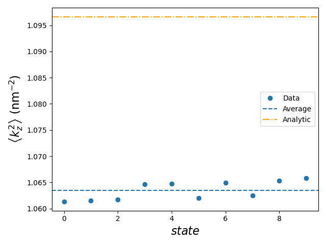
We see that \(\left<k_z^2\right>\) is roughly constant for all 10 states. Furthermore, there is only a \(\sim3\%\) discrepancy between the numerical value (blue dashed line) and the true (analytic) value (orange dot-dashed line):
for the ground-state particle-in-a-box eigenstate. This justifies the projection of the full cubic SOC onto the linear version and using \(\left<k_z^2\right>\) as a constant parameter.
10.6.2. Effect of spin–orbit coupling on the spectrum
Next we compare the spectra as a function of the strength of the applied magnetic field, \(B_0\), with and without spin–orbit coupling. We load the data and then plot the spectra as a function of \(B_0\).
# Energies ---------------------------------------------------------------------

# Load data
SOC_data = np.loadtxt(str(path / "output" / f"{n_soc}.txt"))
no_SOC_data = np.loadtxt(str(path / "output" / f"{n_no_soc}.txt"))

# Plot
fig = plt.figure()
ax1 = fig.add_subplot(1, 1, 1)
ax1.plot(SOC_data[:, 0], SOC_data[:, 1:] * ct.e /meV, marker = "o", linestyle = "-")
ax1.plot(no_SOC_data[:, 0], no_SOC_data[:, 1:] * ct.e/meV, "--")

ax1.set_xlabel(r"$B_0 (T)$", fontsize=16)
ax1.set_ylabel(r"$E$ ($meV$)", fontsize=16)

# Creating legend
dashed = mlines.Line2D([], [], color="black", ls = "--", label="Without SOC")
circle = mlines.Line2D(
   [], [], color="black", marker="o", linestyle="None",
   markersize=10, label="With SOC"
   )
ax1.legend(handles=[dashed, circle])

# Save plot
plt.tight_layout()
plt.savefig(str(path / "output" / f"{n_plot}.png"))
The resulting plot is saved in "output/holes_energies_vs_B.png":
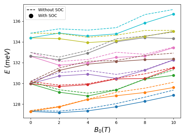
From this plot we can see that the effect of spin–orbit coupling [specifically the spin–orbit coupling of Eq. (10.5.2)] is of the same order as the energy gap between the different bands. For example, the ground state (blue) at \(B_0 = 10 \mathrm{T}\) without spin–orbit coupling is closer to the first excited state (orange) when spin–orbit coupling is included. However qualitatively the spectra with and without spin–orbit coupling have similar features. Therefore, if we only want a qualitative understanding of the spectrum for holes in a GaAs box, it may not be necessary to include spin–orbit coupling in the model. For a quantitative understanding, however, the inclusion of spin–orbit coupling seems necessary.
Note
The spectra presented here could vary depending on the characteristic length of the mesh used. To perform a proper comparison, the calculations should be converged as a function of the characteristic length of the mesh. Nevertheless, the mesh used in this example can give us an idea of the importance of the spin–orbit coupling in this system and allows us to go through an example where both spin–orbit coupling and magnetic effects are included in the calculation in a reasonable amount of time (roughly 10 minutes on a laptop).
10.7. Full code
__copyright__ = "Copyright 2022-2026, Nanoacademic Technologies Inc."

import numpy as np
from matplotlib import pyplot as plt
import matplotlib.lines as mlines
from progress.bar import ChargingBar as Bar
import pathlib
from qtcad.device import materials as mt
from qtcad.device import constants as ct
from qtcad.device.pauli import J_x, J_y
from qtcad.device import Device
from qtcad.device.schrodinger import Solver, SolverParams
from qtcad.device.mesh3d import Mesh

# -------------------------------------------------------------------------------
# Setup
# -------------------------------------------------------------------------------
# Constants
nm = 1e-9
A = 1e-10
meV = ct.e / 1000

# Names of files ---------------------------------------------------------------
path = pathlib.Path(__file__).parent.resolve()

# Output
n_no_soc = "hole_energies_vs_B"
n_soc = "hole_energies_withSOC_vs_B"
n_kz2 = "kz2_holes"
n_plot = "holes_energies_vs_B"

# Input
n_mesh = "box.msh"

# Initialize the meshes --------------------------------------------------------
path_mesh = str(path / "meshes" / f"{n_mesh}")
# Load the mesh
scaling = nm
mesh = Mesh(scaling, path_mesh)

# Create device ------------------------------------------------------------
# Create device from mesh
d = Device(mesh, conf_carriers="h", hole_kp_model="luttinger_kohn_foreman")

# Create regions
d.new_region("domain", mt.GaAs)

# Then create insulator boundaries
d.new_insulator("bnd")

# -------------------------------------------------------------------------------
# Solving Schrodinger Equation with a magnetic field
# -------------------------------------------------------------------------------
print("-------------------------------------------------------")
print("Solving Schrodinger Equation including B field")
print("-------------------------------------------------------")
# Set up solver parameters -------------------------------------------------
# Configure and create the Schrodinger solver
params_schrod = SolverParams()
params_schrod.num_states = 10
params_schrod.verbose = False


# Set up B field ---------------------------------------------------------------
B = 10
B_vec = np.linspace(0, 1, 6) * B
# use a progress bar
progress_bar = Bar("B loop", max=len(B_vec))

data = np.zeros((len(B_vec), params_schrod.num_states + 1))

for i, B0 in enumerate(B_vec):
    # include B in the calculation
    d.set_Bfield(np.array([0, 0, B0]), gauge="landau")

    # Solve --------------------------------------------------------------------
    # Create Schrodinger solver
    ss = Solver(d, solver_params=params_schrod)
    ss.solve()

    # Print results
    print("\n-----------------------------")
    print(f"B = {B0}")
    d.print_energies()
    # Update progress bar
    progress_bar.next()
    print("\n-----------------------------\n")

    # Save results to file
    data[i, 0] = B0
    data[i, 1:] = d.energies / ct.e
    with open(str(path / "output" / f"{n_no_soc}.txt"), "w") as f:
        np.savetxt(f, data)

# -------------------------------------------------------------------------------
# Solving Schrodinger Equation with a magnetic field and SOC
# -------------------------------------------------------------------------------
print("-------------------------------------------------------")
print("Solving Schrodinger Equation including B field and SOC")
print("-------------------------------------------------------")

# Set up SOC -------------------------------------------------------------------
# Compute <k_z^2>
kz2 = np.array([d.get_k_squared(i) for i in range(params_schrod.num_states)])

with open(str(path / "output" / f"{n_kz2}.txt"), "w") as f:
    np.savetxt(f, kz2)

# Coupling coefficient
beta = 82 * ct.e * A**3
# Add SOC to the device
d.set_soc([beta * kz2[0] * J_x, -beta * kz2[0] * J_y, None])

# use a progress bar
progress_bar = Bar("B loop", max=len(B_vec))

data = np.zeros((len(B_vec), params_schrod.num_states + 1))

for i, B0 in enumerate(B_vec):
    # include B in the calculation
    d.set_Bfield(np.array([0, 0, B0]), gauge="landau")

    # Solve --------------------------------------------------------------------
    # Create Schrodinger solver
    ss = Solver(d, solver_params=params_schrod)
    ss.solve()

    # Print results
    print("\n-----------------------------")
    print(f"B = {B0}")
    d.print_energies()
    # Update progress bar
    progress_bar.next()
    print("\n-----------------------------\n")

    # Save results to file
    data[i, 0] = B0
    data[i, 1:] = d.energies / ct.e
    with open(str(path / "output" / f"{n_soc}.txt"), "w") as f:
        np.savetxt(f, data)

# -------------------------------------------------------------------------------
# Plotting
# -------------------------------------------------------------------------------
# <k_z^2> ----------------------------------------------------------------------
kz2_data = np.loadtxt(str(path / "output" / f"{n_kz2}.txt"))

# Analytic value of <k_z^2>
Lz = 3 * nm
kz2_analytic = (np.pi / Lz) ** 2

# Plot
fig = plt.figure()
ax1 = fig.add_subplot(1, 1, 1)
ax1.plot(kz2_data * nm**2, "o", label="Data")
ax1.axhline(np.average(kz2_data) * nm**2, ls="--", label="Average")
ax1.axhline(kz2_analytic * nm**2, ls="-.", color="orange", label="Analytic")

ax1.set_xlabel(r"$state$", fontsize=16)
ax1.set_ylabel(r"$\left<k_z^2\right>$ ($\mathrm{nm}^{-2}$)", fontsize=16)
ax1.legend()

# Save plot
plt.tight_layout()
plt.savefig(str(path / "output" / f"{n_kz2}.png"))

# Energies ---------------------------------------------------------------------

# Load data
SOC_data = np.loadtxt(str(path / "output" / f"{n_soc}.txt"))
no_SOC_data = np.loadtxt(str(path / "output" / f"{n_no_soc}.txt"))

# Plot
fig = plt.figure()
ax1 = fig.add_subplot(1, 1, 1)
ax1.plot(SOC_data[:, 0], SOC_data[:, 1:] * ct.e / meV, marker="o", linestyle="-")
ax1.plot(no_SOC_data[:, 0], no_SOC_data[:, 1:] * ct.e / meV, "--")

ax1.set_xlabel(r"$B_0 (T)$", fontsize=16)
ax1.set_ylabel(r"$E$ ($meV$)", fontsize=16)

# Creating legend
dashed = mlines.Line2D([], [], color="black", ls="--", label="Without SOC")
circle = mlines.Line2D(
    [], [], color="black", marker="o", linestyle="None", markersize=10, label="With SOC"
)
ax1.legend(handles=[dashed, circle])

# Save plot
plt.tight_layout()
plt.savefig(str(path / "output" / f"{n_plot}.png"))