11. Including strain in a simulation

11.1. Requirements

11.1.1. Software components

QTCAD
Gmsh

11.1.2. Geometry file

qtcad/examples/tutorials/meshes/box_order2.geo

11.1.3. Python script

qtcad/examples/tutorials/holes_strain.py

11.1.4. References

11.2. Briefing

In this tutorial, we explain how to include strain in a QTCAD simulation. We will investigate how strain can modify the character of holes confined to a box-like quantum dot. While holes confined to quantum dots are typically found to possess predominantly heavy-hole character, biaxial tensile strain has been shown to lead to ground states with predominantly light-hole character [HWK+14].

The full code may be found at the bottom of this page, or in qtcad/examples/tutorials/holes_strain.py.

11.3. Setting up the device

11.3.1. Header

Like most Python scripts, we start with a header. The header is used to import the relevant modules that will be used in this example.

import numpy as np
from matplotlib import pyplot as plt
import pathlib
from progress.bar import ChargingBar as Bar

from device import materials as mt
from device import constants as ct

from device.mesh3d import Mesh
from device import Device
from device.schrodinger import Solver, SolverParams

The first group of imports are from standard python libraries. The second group contains constants and material properties. The third group of imports contains modules that allow us to create the mesh, the device, and solve the Schrödinger equation.

11.3.2. Setup

After importing the relevant modules, we set up our calculation. This step involves defining constants and creating the mesh and the device over which the simulation will be run.

#-------------------------------------------------------------------------------
# Setup
#-------------------------------------------------------------------------------
# Constants --------------------------------------------------------------------
nm = 1e-9
meV = ct.e/1000

Here we define two constants: nm and meV which, respectively, define the nanometer and the millielectronvolts in SI units. Next, we set up paths to input and output files.

# Names of files ---------------------------------------------------------------
path = pathlib.Path(__file__).parent.resolve()

# Output
n_bw = "holes_strain_bw"
n_energy = "holes_strain_energies"
n_plot = "holes_strain"

# Input
n_mesh = "box_order2.msh2"

The first line defines the path to the script being run. We then define the names of certain output data files and the name of the mesh file that we will load. After the preliminary constants have been defined, we create a Mesh object.

# Initialize the meshes --------------------------------------------------------
path_mesh = str(path/"meshes"/f"{n_mesh}")
# Load the mesh
scaling = nm
mesh = Mesh(scaling, path_mesh)

In this specific example, we are using a second-order mesh (as specified in the corresponding .geo file, ‘box_order2.geo’), from which we then create a Device object.

# Create device ------------------------------------------------------------
# Create device from mesh
d = Device(mesh, conf_carriers="h")
d.hole_kp_model = "luttinger_kohn_foreman"

# Create regions
d.new_region("domain", mt.GaAs)

# Then create insulator boundaries
d.new_insulator("bnd")

The system we have created is a box made of GaAs with dimensions \(60~\mathrm{nm} \times 60~\mathrm{nm} \times 12~\mathrm{nm}\). The device, d, is defined over this box and contains holes as confined carriers, which we model using the 4-band "luttinger_kohn_foreman" model. We have also enforced “insulator” boundary conditions at the faces of the box, which will indicate to the Schrödinger Solver that the wavefunctions should vanish at the boundaries of the box.

11.4. Solving the Schrödinger equation with strain

Now that the Device, d, has been initialized, we can solve the Schrödinger equation. We start by setting up the SolverParams.

#-------------------------------------------------------------------------------
# Solving Schrodinger Equation under biaxial tensile strain
#-------------------------------------------------------------------------------
# Set up solver parameters -----------------------------------------------------
params = SolverParams()
params.num_states = 10

Then, we add biaxial tensile strain to the system. The strain tensor has components \(\varepsilon_{xx} > 0\) and \(\varepsilon_{yy} > 0\) with all other components vanishing. We will solve the Schrödinger equation for different magnitudes of the strain \(\varepsilon_{xx}=\varepsilon_{yy}\). The different magnitudes are stored in the array R.

# Set up strain ----------------------------------------------------------------
# Biaxial tensile strain
R = np.linspace(0, 0.01, 5)
strain = np.array([
            [1, 0, 0],
            [0, 1, 0],
            [0, 0, 0]
        ])
# use a progress bar
progress_bar = Bar("Strain loop", max = len(R))

In the above snippet we have also set up a progress bar, Bar, to track the calculation. We loop over the different values of strain. For each generated strain tensor, we use the set_strain method to set the tensor over the Device, d. This method takes as input a 2D numpy array representing the homogenous strain affecting the entire device. In this case, this array is given by r * strain.

nrg = []
bw = []

for r in R:
    # Set strain
    d.set_strain(r * strain)

    # Solve --------------------------------------------------------------------
    # Create Schrodinger solver
    s = Solver(d, solver_params=params)
    s.solve()

    # Print results
    print('------------------------')
    print(f'e_xx = e_yy = {r}')
    d.print_energies()
    progress_bar.next() # Update progress bar
    print('\n------------------------')

    # Store energies
    nrg.append(d.energies)
    # Store band weights
    bw.append(d.band_weight())

# Finish progress bar
progress_bar.finish()

# Save data --------------------------------------------------------------------
# Energy
nrg = np.array(nrg)
E = np.zeros((nrg.shape[0], nrg.shape[1]+1))
E[:, 0] = R
E[:, 1:] = nrg
np.savetxt(str(path/"data"/f"{n_energy}.txt"), E)
# Band weights
bw = np.array(bw)
BW = np.zeros((bw.shape[0], bw.shape[1], 2))
BW[..., 0] = bw[..., 0] + bw[..., 1] # Heavy hole weight
BW[..., 1] = bw[..., 2] + bw[..., 3] # Light hole weight
np.savetxt(str(path/"data"/f"{n_bw}.txt"), BW[:, 0, :])

After setting the strain, we create a Schrödinger Solver and solve the Schrödinger equation. We then append the energies to the nrg list. We also use the band_weight method to compute the contribution from each band (2 heavy-hole and 2 light-hole bands) to each eigenstate and append the output to the bw list. Specifically, the band_weight method outputs a 2D numpy array. The entries in this array are \(\left|\left<3/2, \nu| j\right>\right|^2\), where \(\left| j\right>\) is the \(j^{\mathrm{th}}\) eigenstate of the system and \(\left|3/2, \nu\right>\) is a state at the valence-band extremum (in our case \(\nu\) runs over the ordered set \(\{+3/2, -3/2, +1/2, -1/2\}\), i.e., the heavy-hole and light-hole states respectively). The first index of the array runs over the different eigenstates (labelled by \(j\) above) and the second runs over the different valence bands of the "luttinger_kohn_foreman" model we are considering (labelled by \(\nu\) above).

The goal of this loop is to compute the band weights as a function of the magnitude of the applied biaxial tensile strain. We expect a transition from predominantly heavy-hole-like ground state to predominantly light-hole-like ground state to occur for some value of strain \(\varepsilon_{xx}=\varepsilon_{yy}\) between 0 and 0.01. After the loop is complete, the energies for different values of strain are saved to "data/holes_strain_energies.txt" and the heavy-hole and light-hole weights are saved to "data/holes_strain_bw.txt".

Note

There are 2 heavy-hole bands and 2 light-hole bands. The band_weight method therefore computes four weights for each eigenstate. However, because we are only interested in the relative weights of heavy and light holes, we store the total heavy-hole (sum over the 2 separate heavy-hole weights) and total light-hole (sum over the 2 separate light-hole weights) contributions in BW.

Note

The set_strain method can also be used to analyze the effects of inhomogeneous strain. In the current example, the focus is on homogeneous strain and therefore we pass a single numpy array to the set_strain method. Alternatively, we could pass a function of three variables, each representing a spatial dimension (x, y, and z) which outputs a 2D, \(3\times 3\) numpy array. This function can be used to define the strain at every position in space.

11.5. Visualizing results

Finally, we visualize the results. We plot the eigenenergies of the system as a function of the applied strain as well as the heavy-hole and light-hole weights associated with the ground state as a function of the applied strain.

#-------------------------------------------------------------------------------
# Plotting
#-------------------------------------------------------------------------------
# Create plot
fig = plt.figure()
# Plot energies
ax1 = fig.add_subplot(2, 1, 1)
ax1.plot(E[:, 0], E[:, 1:]/meV)
ax1.set_xlabel(
    r'biaxial strain, $\varepsilon_{xx} = \varepsilon_{yy}$', fontsize=14
    )
ax1.set_ylabel(r'$E$ ($meV$)', fontsize=14)
# Plot band weights
ax2 = fig.add_subplot(2, 1, 2)
ax2.plot(E[:, 0], BW[:, 0, 0], label="HH weight")
ax2.plot(E[:, 0], BW[:, 0, 1], label="LH weight")
ax2.set_xlabel(
    r'biaxial strain, $\varepsilon_{xx} = \varepsilon_{yy}$', fontsize=14
    )
ax2.set_ylabel(r'ground-state weights', fontsize=14)
ax2.legend()

# Save plot
plt.tight_layout()
plt.savefig(str(path / "output" / f"{n_plot}.png"))

The plots are saved in "output/holes_strain.png"

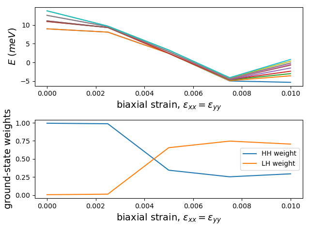
We see that at roughly \(\varepsilon_{xx}=\varepsilon_{yy} \simeq 0.004\) there is a transition between a predominantly heavy-hole ground state (blue line) to a predominantly light-hole ground state (orange line). This transition is consistent with the Fig. 4 of [HWK+14].

Note

The results presented here could vary depending on the characteristic length of the mesh used. To perform a proper comparison, the calculations should be converged as a function of the characteristic length of the mesh. Nevertheless, the mesh used in this example can give us an idea of where to expect the heavy-hole-to-light-hole transition.

11.6. Full code

__copyright__ = "Copyright 2023, Nanoacademic Technologies Inc."

import numpy as np
from matplotlib import pyplot as plt
import pathlib
from progress.bar import ChargingBar as Bar
from device import materials as mt
from device import constants as ct
from device.mesh3d import Mesh
from device import Device
from device.schrodinger import Solver, SolverParams

#-------------------------------------------------------------------------------
# Setup
#-------------------------------------------------------------------------------
# Constants --------------------------------------------------------------------
nm = 1e-9
meV = ct.e/1000

# Names of files ---------------------------------------------------------------
path = pathlib.Path(__file__).parent.resolve()

# Output
n_bw = "holes_strain_bw"
n_energy = "holes_strain_energies"
n_plot = "holes_strain"

# Input
n_mesh = "box_order2.msh2"

# Initialize the meshes --------------------------------------------------------
path_mesh = str(path/"meshes"/f"{n_mesh}")
# Load the mesh
scaling = nm
mesh = Mesh(scaling, path_mesh)

# Create device ------------------------------------------------------------
# Create device from mesh
d = Device(mesh, conf_carriers="h")
d.hole_kp_model = "luttinger_kohn_foreman"

# Create regions
d.new_region("domain", mt.GaAs)

# Then create insulator boundaries
d.new_insulator("bnd")

#-------------------------------------------------------------------------------
# Solving Schrodinger Equation under biaxial tensile strain
#-------------------------------------------------------------------------------
# Set up solver parameters -----------------------------------------------------
params = SolverParams()
params.num_states = 10  

# Set up strain ----------------------------------------------------------------
# Biaxial tensile strain
R = np.linspace(0, 0.01, 5)
strain = np.array([
            [1, 0, 0],
            [0, 1, 0],
            [0, 0, 0]
        ])
# use a progress bar
progress_bar = Bar("Strain loop", max = len(R))

nrg = []
bw = []

for r in R:
    # Set strain
    d.set_strain(r * strain)

    # Solve --------------------------------------------------------------------
    # Create Schrodinger solver 
    s = Solver(d, solver_params=params)
    s.solve()

    # Print results
    print('------------------------')
    print(f'e_xx = e_yy = {r}')
    d.print_energies()
    progress_bar.next() # Update progress bar
    print('\n------------------------')

    # Store energies
    nrg.append(d.energies)
    # Store band weights
    bw.append(d.band_weight())

# Finish progress bar
progress_bar.finish()

# Save data --------------------------------------------------------------------
# Energy
nrg = np.array(nrg)
E = np.zeros((nrg.shape[0], nrg.shape[1]+1))
E[:, 0] = R
E[:, 1:] = nrg
np.savetxt(str(path/"data"/f"{n_energy}.txt"), E)
# Band weights
bw = np.array(bw)
BW = np.zeros((bw.shape[0], bw.shape[1], 2))
BW[..., 0] = bw[..., 0] + bw[..., 1] # Heavy hole weight
BW[..., 1] = bw[..., 2] + bw[..., 3] # Light hole weight
np.savetxt(str(path/"data"/f"{n_bw}.txt"), BW[:, 0, :])

#-------------------------------------------------------------------------------
# Plotting
#-------------------------------------------------------------------------------
# Create plot
fig = plt.figure()
# Plot energies
ax1 = fig.add_subplot(2, 1, 1)
ax1.plot(E[:, 0], E[:, 1:]/meV)
ax1.set_xlabel(
    r'biaxial strain, $\varepsilon_{xx} = \varepsilon_{yy}$', fontsize=14
    )
ax1.set_ylabel(r'$E$ ($meV$)', fontsize=14)
# Plot band weights
ax2 = fig.add_subplot(2, 1, 2)
ax2.plot(E[:, 0], BW[:, 0, 0], label="HH weight")
ax2.plot(E[:, 0], BW[:, 0, 1], label="LH weight")
ax2.set_xlabel(
    r'biaxial strain, $\varepsilon_{xx} = \varepsilon_{yy}$', fontsize=14
    )
ax2.set_ylabel(r'ground-state weights', fontsize=14)
ax2.legend()

# Save plot
plt.tight_layout()
plt.savefig(str(path / "output" / f"{n_plot}.png"))