19. Exchange coupling in a double quantum dot in FD-SOI—Part 2: Exact diagonalization
19.1. Requirements
19.1.1. Software components
QTCAD
Gmsh
19.1.2. Geometry file
qtcad/examples/tutorials/meshes/dqdfdsoi.geo
19.1.3. Python script
qtcad/examples/tutorials/exchange_2.py
19.1.4. References
A double quantum dot device in a fully-depleted silicon-on-insulator transistor
Tunnel coupling in a double quantum dot in FD-SOI—Part 1: Plunger gate tuning
Tunnel coupling in a double quantum dot in FD-SOI—Part 2: Tuning the barrier gate
Exchange coupling in a double quantum dot in FD-SOI—Part 1: Perturbation theory
19.2. Briefing
In Exchange coupling in a double quantum dot in FD-SOI—Part 1: Perturbation theory, we considered a simple analytic expression of the exchange interaction strength which was derived from the Fermi–Hubbard Hamiltonian using perturbation theory. This expression was used to estimate the exchange interaction strength from two parameters that may be obtained from single-electron properties: the double dot tunnel coupling \(\Omega\) and the on-site Coulomb interaction strength \(U\).
In this tutorial, we go beyond this approximate perturbative treatment by using the exact diagonalization method to calculate the exchange interaction strength, as explained in the Exchange interaction through exact diagonalization theory section. Contrary to previous tutorials, which may be executed on a laptop within minutes, this tutorial is much more computationally expensive. In particular, computing the Coulomb integrals may be quite time consuming. Therefore, to execute the current tutorial, we recommend using a workstation that contains enough CPU cores to run at least 16 threads in parallel.
19.3. Header
We start by importing the necessary packages, classes, and functions.
import numpy as np
import pathlib
from timeit import default_timer as timer
from qtcad.device import constants as ct
from qtcad.device import io
from qtcad.device.mesh3d import Mesh, SubMesh
from qtcad.device import materials as mt
from qtcad.device import Device, SubDevice
from qtcad.device.poisson import SolverParams as PoissonSolverParams
from qtcad.device.poisson import Solver as PoissonSolver
from qtcad.device.schrodinger import SolverParams as SchrodingerSolverParams
from qtcad.device.schrodinger import Solver as SchrodingerSolver
from qtcad.device.many_body import Solver as ManyBodySolver
from qtcad.device.many_body import SolverParams as ManyBodySolverParams
from helper.double_dot_fdsoi import get_double_dot_fdsoi
These packages, classes, and functions were all seen in previous tutorials.
19.4. Setting up the device
Again, we start by setting up the paths for the input mesh and for the output files.
# Set up paths
script_dir = pathlib.Path(__file__).parent.resolve()
path_mesh = script_dir / "meshes"
path_out = script_dir / "output"
We then load the outcome of the perturbative calculation of Exchange coupling in a double quantum dot in FD-SOI—Part 1: Perturbation theory for future comparison with the exact diagonalization approach taken below.
# Load the perturbative value of the exchange coupling from a previous
# calculation
path_exchange_perturbation = path_out / "exchange_perturbation.txt"
exchange_perturbation = np.loadtxt(path_exchange_perturbation)
We then load the mesh, again using the final refined mesh from the adaptive calculation done in Tunnel coupling in a double quantum dot in FD-SOI—Part 1: Plunger gate tuning.
# Load the mesh
scaling = 1e-9
path_file = str(path_mesh / "refined_dqdfdsoi.msh")
mesh = Mesh(scaling, path_file)
In this tutorial, as in Exchange coupling in a double quantum dot in FD-SOI—Part 1: Perturbation theory, we will use the bias configuration of Tunnel coupling in a double quantum dot in FD-SOI—Part 2: Tuning the barrier gate that gave the strongest tunnel coupling. This is to maximize the exchange interaction strength. Indeed, we expect larger values of exchange to be computed with lower relative error and to therefore be able to compute a reasonably accurate value of exchange even for coarse meshes and small basis sets. Therefore, due to the smaller computational resource requirements, this large exchange configuration is more appropriate for a tutorial.
We use the same gate bias configuration as in this tutorial, except that we do not include the numerical offset of plunger gate 2 that was computed in Tunnel coupling in a double quantum dot in FD-SOI—Part 1: Plunger gate tuning for the weakest tunnel coupling. This is not necessary here, since the artificial double dot detuning that results from mesh asymmetry is negligible compared with the strongest value of tunnel coupling found in Tunnel coupling in a double quantum dot in FD-SOI—Part 2: Tuning the barrier gate. For weaker tunneling, however, including a numerical offset may be necessary.
# Define the gate biases
back_gate_bias = -0.5
barrier_gate_1_bias = 0.5
plunger_gate_1_bias = 0.59
barrier_gate_2_bias = 0.57
plunger_gate_2_bias = 0.59
barrier_gate_3_bias = 0.5
After setting variable values
for the gate biases, we define the Device
using get_double_dot_fdsoi and create a
SubMesh for the double quantum dot
region.
# Define the device
dvc = get_double_dot_fdsoi(mesh, back_gate_bias, barrier_gate_1_bias,
    plunger_gate_1_bias, barrier_gate_2_bias, plunger_gate_2_bias,
    barrier_gate_3_bias)

# List of regions forming the double quantum dot region
dot_region_list = ["oxide_dot", "gate_oxide_dot", "buried_oxide_dot",
                    "channel_dot"]

# Create the submesh object for the dot region
submesh = SubMesh(dvc.mesh, dot_region_list)
19.5. Electrostatics and single-electron eigenstates
As usual, the next step is to compute the electric potential throughout the
device using the non-linear Poisson solver. To do so, we load the potential
that was obtained in Tunnel coupling in a double quantum dot in FD-SOI—Part 1: Plunger gate tuning into the device, configure
the non-linear Poisson solver parameters, instantiate the Poisson
Solver object,
and run it using its
solve
method with the optional argument initialize set to False to use
the electric potential stored in the device as an initial guess.
# Load the electric potential from the previous run to speed up Poisson
# calculation
phi = io.load(path_out / "tunnel_coupling_final_potential.hdf5",
    var_name="phi")
dvc.set_potential(phi)

# Configure the non-linear Poisson solver
params_poisson = PoissonSolverParams()
params_poisson.tol = 1e-3 # Convergence threshold (tolerance) for the error

# Instantiate Poisson solver
poisson_slv = PoissonSolver(dvc, solver_params=params_poisson)

# Solve Poisson's equation
poisson_slv.solve(initialize=False)
We next configure the single-electron Schrödinger solver, set the confinement
potential from the electric potential obtained from the non-linear Poisson
solution, create a
SubDevice object for the double quantum
dot region, instantiate a Schrödinger
Solver object, call its
solve method,
and print the resulting eigenenergies.
# Configure the Schrödinger solver
params_schrod = SchrodingerSolverParams()
params_schrod.tol = 1e-6      # Tolerance on energies in eV

# Get the potential energy from the band edge for usage in the Schrodinger
# solver
dvc.set_V_from_phi()

# Create a subdevice for the dot region
subdvc = SubDevice(dvc, submesh)

# Create a Schrodinger solver, and run it
schrod_solver = SchrodingerSolver(subdvc, solver_params=params_schrod)
schrod_solver.solve()
subdvc.print_energies()
We get
Energy levels (eV)
[0.04332927 0.04358678 0.04831340 0.04857437 0.05149798 0.05495186
 0.05513753 0.05540500 0.05650954 0.05999599]
19.6. Exact diagonalization of the two-electron Hamiltonian
We first create a many-body
SolverParams
object to configure the exact diagonalization method, and use it in the
instantiation of a many-body
Solver object.
# Solving the many-body hamiltonian
# Instantiate many-body solver
manybody_solver_params = ManyBodySolverParams()
manybody_solver_params.n_degen = 2
manybody_solver_params.num_states = 8
manybody_solver_params.num_particles = [2]
manybody_solver_params.overlap = True
manybody_solver = ManyBodySolver(subdvc,
    solver_params=manybody_solver_params)
We use n_degen = 2 to account for spin degeneracy. In addition, we set
num_states = 8, meaning that the first 8 spin-degenerate single-electron
eigenstates are used as a basis set to construct the many-body Hamiltonian
(bringing the total number of basis states to \(8\times2 = 16\)).
We found that for the current gate bias configuration, smaller basis sets
are not sufficiently accurate. Larger basis sets would be more accurate,
but also lead to much longer computation times. In addition, we set
num_particles = [2] to indicate that we are only interested in the
two-particle subspace of the many-body Hamiltonian, and set
overlap = True to indicate that we will keep all the terms in the
four-dimensional Coulomb integrals matrix. Setting overlap to False
would greatly speed up calculations, but we found this to also lead to
results that are incorrect by several orders of magnitude.
Having set up the many-body solver, we run its
solve method.
# Solve the many-body hamiltonian
t0 = timer()
manybody_solver.solve()
print("Two-electron solution found in {} s".format(timer()-t0))
In addition, we use the default timer of the
timeit
module to measure the computation time. When writing this tutorial, we
completed this part of the calculation in approximately 5 minutes on a
Lenovo Thinkpad X13 with an 11th Gen Intel Core i7-1185G7 CPU @ 2.40GHz
(4 cores, 8 threads) and 16 GB of RAM.
Because this exchange calculation allows us to concentrate on the two-electron
subspace, construction and diagonalization of the many-body Hamiltonian is
not a computational bottleneck. In fact, almost all the computation time is
spent in the calculation of Coulomb integrals, for which brute-force
integration methods would lead to a computational complexity of
\(O(N^4)\) for \(N\) basis states. In QTCAD, we leverage a filtering
technique to drop negligible integrals. In the absence of any memory
limitations, this approach can achieve a computational complexity
of \(O(N^2)\). See the many-body
SolverParams API reference
for more details on how to configure the filtering algorithm and control
memory usage.
19.7. Exchange interaction strength
Once the many-body problem is solved, we may readily calculate the exchange interaction strength.
We first extract the two-electron eigenenergies from the above calculations
by calling the
get_N_particle_subspace
method
of the Device class. After printing the
first eight eigenenergies, we save all the energies in a text file.
# Get the two-electron eigenenergies
two_electron_energies = subdvc.get_N_particle_subspace(2).eigval/ct.e
print("Two-electron energies")
print(two_electron_energies[0:8])
np.savetxt(path_out/"exchange_two_electron_energies.txt", two_electron_energies)
For the first eight eigenenergies, we get:
Two-electron energies
[0.09088798 0.09089042 0.09089042 0.09089042 0.09560985 0.09560985
 0.09560985 0.09561834]
As expected, we find a singlet (non-degenerate) ground state, and a triply-degenerate (triplet) first excited state.
The exchange interaction strength is given simply by the energy difference between the singlet and triplet states.
# Calculate the exchange interaction strength
exchange = two_electron_energies[1] - two_electron_energies[0]
Finally, we print the exchange interaction strength in MHz, and compare it with the value obtained from perturbation theory in the previous tutorial.
# Print the output, and compare it with perturbation theory
print ('Exchange coupling (exact diagonalization): {:.3f} MHz'\
    .format(exchange*ct.e/ct.h/1e6))
print ('Exchange coupling (perturbation theory): {:.3f} MHz'\
    .format(exchange_perturbation/ct.h/1e6))
We get:
Exchange coupling (exact diagonalization): 590.204 MHz
Exchange coupling (perturbation theory): 929.216 MHz
For the current gate bias configuration, solver parameters, and mesh, perturbation theory is in agreement with the exact diagonalization approach within a relative error of roughly 45 %. Despite this significant discrepancy, the order of magnitude of the exact and perturbative approaches agree. Indeed, here, we have purposefully kept the basis set and mesh size small to allow for a short computation time compatible with a tutorial. As will be seen in the next section, agreement between the two techniques improves as the basis set dimension and mesh size are increased.
19.8. Convergence analysis
Since the perturbative approach is approximate, we cannot expect it to agree with exact diagonalization, in general. Conditions under which the perturbative approach is expected to be accurate in principle are given in Perturbation theory of exchange coupling in a double quantum dot. Beyond these parametric regimes, for this method to be accurate, finite-element simulations employed to calculate the tunnel coupling and the Coulomb interaction strength must also be converged with respect to mesh refinements.
In addition, despite its name, the exact diagonalization approach is only perfectly accurate for infinitely fine meshes and infinitely large single-electron basis sets. In practice, an increasingly fine mesh and an increasingly large number of basis states are observed to be required for convergence as the exchange interaction strength is decreased.
Therefore, here, we show a convergence analysis of both the exact diagonalization and perturbative approaches with respect to the mesh characteristic length and the number of orbital basis states. The results of this convergence analysis are summarized in the plots below.
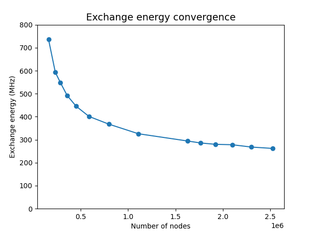
Fig. 19.8.1 Convergence of the exchange interaction strength with mesh characteristic
length. In these calculations, we set the num_states parameter of
the many-body SolverParams
object to 12, and tune the h_refined parameter
of the non-linear Poisson
SolverParams object
over fourteen values between 0.8 and 0.3. This enables to refine the mesh
within the quantum dot region only.
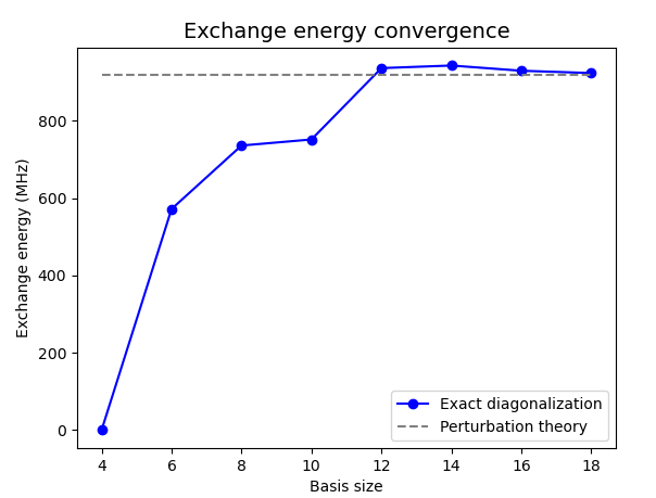
Fig. 19.8.2 Convergence of the exchange interaction strength with the dimension of
the single-electron basis set. In all these simulations, we set the
h_refined parameter of the non-linear Poisson
SolverParams object
to 0.4 and tune the num_states parameter of
the many-body SolverParams
object over 8 values between 4 and 18. For num_states = 4, we find that
the ground state is triply degenerate and the first excited state is a
singlet, which is a clear sign that the basis set is insufficiently large
(for this data point, we illustrate this anomaly by setting exchange to
zero in the plot).
Indeed, we expect the exchange interaction to lower the singlet state
energy with respect to the triplet states in all realistic gated quantum
dots.
We observe that the exact diagonalization approach converges to a fixed value as the basis size is increased which is consistent with the predictions of perturbation theory made in Exchange coupling in a double quantum dot in FD-SOI—Part 1: Perturbation theory.
Note
The QTCAD scripts used to generate the above convergence plots are not
included in this tutorial. However, they are available in the
examples/tutorials/conv_exchange directory which is shipped with
the QTCAD code.
19.9. Full code
__copyright__ = "Copyright 2022-2026, Nanoacademic Technologies Inc."

import numpy as np
import pathlib
from timeit import default_timer as timer
from qtcad.device import constants as ct
from qtcad.device import io
from qtcad.device.mesh3d import Mesh, SubMesh
from qtcad.device import materials as mt
from qtcad.device import Device, SubDevice
from qtcad.device.poisson import SolverParams as PoissonSolverParams
from qtcad.device.poisson import Solver as PoissonSolver
from qtcad.device.schrodinger import SolverParams as SchrodingerSolverParams
from qtcad.device.schrodinger import Solver as SchrodingerSolver
from qtcad.device.many_body import Solver as ManyBodySolver
from qtcad.device.many_body import SolverParams as ManyBodySolverParams
from helper.double_dot_fdsoi import get_double_dot_fdsoi

# Set up paths
script_dir = pathlib.Path(__file__).parent.resolve()
path_mesh = script_dir / "meshes"
path_out = script_dir / "output"

# Load the perturbative value of the exchange coupling from a previous
# calculation
path_exchange_perturbation = path_out / "exchange_perturbation.txt"
exchange_perturbation = np.loadtxt(path_exchange_perturbation)

# Load the mesh
scaling = 1e-9
path_file = str(path_mesh / "refined_dqdfdsoi.msh")
mesh = Mesh(scaling, path_file)

# Define the gate biases
back_gate_bias = -0.5
barrier_gate_1_bias = 0.5
plunger_gate_1_bias = 0.59
barrier_gate_2_bias = 0.57
plunger_gate_2_bias = 0.59
barrier_gate_3_bias = 0.5

# Define the device
dvc = get_double_dot_fdsoi(
    mesh,
    back_gate_bias,
    barrier_gate_1_bias,
    plunger_gate_1_bias,
    barrier_gate_2_bias,
    plunger_gate_2_bias,
    barrier_gate_3_bias,
)

# List of regions forming the double quantum dot region
dot_region_list = ["oxide_dot", "gate_oxide_dot", "buried_oxide_dot", "channel_dot"]

# Create the submesh object for the dot region
submesh = SubMesh(dvc.mesh, dot_region_list)

# Load the electric potential from the previous run to speed up Poisson
# calculation
phi = io.load(path_out / "tunnel_coupling_final_potential.hdf5", var_name="phi")
dvc.set_potential(phi)

# Configure the non-linear Poisson solver
params_poisson = PoissonSolverParams()
params_poisson.tol = 1e-3  # Convergence threshold (tolerance) for the error

# Instantiate Poisson solver
poisson_slv = PoissonSolver(dvc, solver_params=params_poisson)

# Solve Poisson's equation
poisson_slv.solve(initialize=False)

# Configure the Schrödinger solver
params_schrod = SchrodingerSolverParams()
params_schrod.tol = 1e-6  # Tolerance on energies in eV

# Get the potential energy from the band edge for usage in the Schrodinger
# solver
dvc.set_V_from_phi()

# Create a subdevice for the dot region
subdvc = SubDevice(dvc, submesh)

# Create a Schrodinger solver, and run it
schrod_solver = SchrodingerSolver(subdvc, solver_params=params_schrod)
schrod_solver.solve()
subdvc.print_energies()

# Solving the many-body hamiltonian
# Instantiate many-body solver
manybody_solver_params = ManyBodySolverParams()
manybody_solver_params.n_degen = 2
manybody_solver_params.num_states = 8
manybody_solver_params.num_particles = [2]
manybody_solver_params.overlap = True
manybody_solver = ManyBodySolver(subdvc, solver_params=manybody_solver_params)

# Solve the many-body hamiltonian
t0 = timer()
manybody_solver.solve()
print("Two-electron solution found in {} s".format(timer() - t0))

# Get the two-electron eigenenergies
two_electron_energies = subdvc.get_N_particle_subspace(2).eigval / ct.e
print("Two-electron energies")
print(two_electron_energies[0:8])
np.savetxt(path_out / "exchange_two_electron_energies.txt", two_electron_energies)

# Calculate the exchange interaction strength
exchange = two_electron_energies[1] - two_electron_energies[0]

# Print the output, and compare it with perturbation theory
print(
    "Exchange coupling (exact diagonalization): {:.3f} MHz".format(
        exchange * ct.e / ct.h / 1e6
    )
)
print(
    "Exchange coupling (perturbation theory): {:.3f} MHz".format(
        exchange_perturbation / ct.h / 1e6
    )
)