14. Many-body analysis of a nanowire quantum dot
14.1. Requirements
14.1.1. Software components
qtcad
gmsh
14.1.2. Geometry file
qtcad/examples/tutorials/meshes/nanowire.geo
14.1.3. Python script
qtcad/examples/tutorials/manybody.py
14.1.4. References
14.2. Briefing
In this tutorial, we build on the results output in the Poisson and Schrödinger simulation of a nanowire quantum dot
tutorial (see Python script qtcad/examples/tutorials/nanowire.py).
Loading the potential obtained at the end of this file, we solve the
many-body problem for a system consisting of a few electrons confined in the
potential well formed by the conduction band edge within the channel of the
nanowire quantum dot. We then illustrate the various physical outputs that
can be extracted from the many-body solution.
14.3. Setting up the device and loading results from the previous simulation
14.3.1. Header
The header for this tutorial is
from qtcad.device import constants as ct
from qtcad.device.mesh3d import Mesh
from qtcad.device import io
from qtcad.device import analysis as an
from qtcad.device import materials as mt
from qtcad.device import Device
from qtcad.device.schrodinger import Solver as SingleBodySolver
import pathlib
from qtcad.device.many_body import Solver as ManyBodySolver
from qtcad.device.many_body import SolverParams
The only new additions with respect to the Poisson and Schrödinger simulation of a nanowire quantum dot tutorial are the
last two lines of the code block, in which the many-body
Solver and
SolverParams
classes are imported from the
many_body module.
14.3.2. Creating the device
We next load the mesh, instantiate the device, and set up regions and boundary conditions exactly as in the previous tutorial.
# Define some device parameters
Vgs = 0.5 # Gate-source bias
Ew = mt.Si.chi + mt.Si.Eg/2 # Metal work function
Ltot = 20e-9 # Device height in m
radius = 2.5e-9 # Device radius in m

# Paths to mesh file and output files
script_dir = pathlib.Path(__file__).parent.resolve()
path_mesh = script_dir / "meshes/" / "nanowire.msh"
path_hdf5 = script_dir / "output/" / "nanowire.hdf5"

# Load the mesh
scaling = 1e-9
mesh = Mesh(scaling, str(path_mesh))

# Create device from mesh and set statistics.
# It is important to set statistics before creating boundaries since
# they determine the boundary values, Failing to do so will produce
# inconsistent results.
dvc = Device(mesh, conf_carriers="e")
dvc.statistics = "FD_approx"  # Analytic approximation to Fermi-Dirac statistics

# Create regions first.
# Make sure each element is assigned to a region, otherwise default
# (silicon) parameters are used
dvc.new_region('channel_ox',mt.SiO2)
dvc.new_region('source_ox',mt.SiO2)
dvc.new_region('drain_ox',mt.SiO2)
dvc.new_region('channel', mt.Si)
dvc.new_region('source', mt.Si, pdoping=5e20*1e6, ndoping=0)
dvc.new_region('drain', mt.Si, pdoping=5e20*1e6, ndoping=0)

# Then create boundaries
dvc.new_ohmic_bnd('source_bnd')
dvc.new_ohmic_bnd('drain_bnd')
dvc.new_gate_bnd('gate_bnd',Vgs,Ew)
The next step is to load the electric potential from the hdf5 output file produced in the previous tutorial.
# Load the electic potential
dvc.set_potential(io.load(path_hdf5,"phi"))
It is important to use the
set_potential
method of the
Device class rather than modifying the
phi attribute directly because the
method automatically recalculates the potential energy
V.
14.4. Solving the many-body problem
We first solve the single-electron problem, which will define the single-particle basis set for the many-body problem
# Solve the single-electron problem
slv = SingleBodySolver(dvc)
slv.solve()
dvc.print_energies()
The single-particle energies will be output as
Energy levels (eV)
[0.54798018 0.61320021 0.68496646 0.76317642 0.8478653  0.93920254
1.03757746 1.14369621 1.15198013 1.15240696]
We then instantiate and run the many-body
Solver.
# Solve the many-body problem
solver_params = SolverParams()
solver_params.num_states = 3
solver_params.n_degen = 2
solver_params.alpha = 0.5
solver_params.num_particles = [0,1,2,3]
slv = ManyBodySolver(dvc, solver_params = solver_params)
slv.solve()
Here we limit the number of single-particle orbitals to consider in the basis
set to \(3\), and set the degeneracy of these orbitals to
\(2`\) (e.g. from spin). In addition, we introduce a lever arm
\(\alpha\) of \(0.5\). The lever arm quantifies the extent by which
a potential applied at a gate can shift the energy-level structure of the
device (see the lever arm Theory section). Finally,
we set the num_particles attribute of the many-body
SolverParams to a list of
integers \(N\) labeling the
\(N\)-particle subspaces to consider. Here, we choose to only consider the
0-, 1-, 2-, and 3-particle subspaces even though for
\(n_\mathrm{states} = 3\) and \(n_\mathrm{degen} = 2\),
the maximum number of particles that can be considered in principle is
\(n_\mathrm{states} \times n_\mathrm{degen} = 6\).
This choice is up to the user, but taking a smaller number of particles than
the total accessible amount will typically make calculations faster.
After calling the
solve method,
progress bars appear to track the calculation of Coulomb integrals
Initializing Coulomb matrix calculation. ████████████████████████████████ 100%
Computing contributions to block-row 0 (part 1/2) ████████████████████████████████ 100%
Computing contributions to block-row 1 (part 1/2) ████████████████████████████████ 100%
Computing contributions to block-row 2 (part 1/2) ████████████████████████████████ 100%
Computing contributions to block-row 0 (part 2/2) ████████████████████████████████ 100%
Computing contributions to block-row 1 (part 2/2) ████████████████████████████████ 100%
Computing contributions to block-row 2 (part 2/2) ████████████████████████████████ 100%
Computing Coulomb integrals...
Done.
14.5. Analyzing the results
Once the calculation is done, we produce various outputs that are made
available through quantities stored as new
Device
attributes.
14.5.1. Many-body subspace properties
We first analyze the many-body subspaces with
# Many-body subspace properties
print("Many-body subspaces:", dvc.many_body_subspaces)
print("Number of subspaces:", len(dvc.many_body_subspaces))
print("Electron number in subspace 2:", dvc.many_body_subspaces[2].N)
which results in
Many-body subspaces: [<device.core.quantum.Subspace object at 0x00000215769AD6A0>, <device.core.quantum.Subspace object at 0x0000021576CC1E80>, <device.core.quantum.Subspace object at 0x0000021576CC1FA0>, <device.core.quantum.Subspace object at 0x0000021576CC1E20>]
Number of subspaces: 4
Electron number in subspace 2: 2
In general, for \(n_\mathrm{states}=3\) single-particle orbitals with degeneracy \(n_\mathrm{degen}=2\), we have \(n_\mathrm{states}\times n_\mathrm{degen}+1=7\) subspaces corresponding to \(0\) to \(N_\mathrm{max}=n_\mathrm{states}\times n_\mathrm{degen}=6\) electrons (see Exact diagonalization). However, here, we have kept only the 0, 1, 2, and 3-electron subspaces. With these subspace integer labels starting at 0, the many-body subspace with index 2 is indeed expected to involve 2 electrons, as seen above.
Each subspace contains a many-body basis set. For example, the two-electron subspace basis set is displayed with
print("Two-electron many-body basis set (integers): ")
print(dvc.get_N_particle_subspace(2).get_bas_set())
which results in
Two-electron many-body basis set (integers):
[ 3  5  9 17 33  6 10 18 34 12 20 36 24 40 48]
By default, each many-body basis state is labeled by an integer whose binary
representation gives the occupation (0 if unoccupied, 1 if occupied) of each
single-partical orbital (see the
get_bas_set
API reference). This is the most compact representation available in QTCAD®
in terms of memory usage. The strings for these binaries may be displayed with:
print("Two-electron many-body basis set (binary strings): ")
print(dvc.get_N_particle_subspace(2).get_bas_set(dtype="str"))
which results in
Two-electron many-body basis set (binary strings):
['000011' '000101' '001001' '010001' '100001' '000110' '001010' '010010'
'100010' '001100' '010100' '100100' '011000' '101000' '110000']
We remark that these strings must be read from right to left when converting into orbital occupations. The above basis set may be written as an array of integers whose rows correspond to many-body basis states and columns to single-particle orbitals with
print("Two-electron many-body basis set (array): ")
print(dvc.get_N_particle_subspace(2).get_bas_set(dtype="array"))
which results in
Two-electron many-body basis set (array):

[[1 1 0 0 0 0]
[1 0 1 0 0 0]
[1 0 0 1 0 0]
[1 0 0 0 1 0]
[1 0 0 0 0 1]
[0 1 1 0 0 0]
[0 1 0 1 0 0]
[0 1 0 0 1 0]
[0 1 0 0 0 1]
[0 0 1 1 0 0]
[0 0 1 0 1 0]
[0 0 1 0 0 1]
[0 0 0 1 1 0]
[0 0 0 1 0 1]
[0 0 0 0 1 1]]
This corresponds to all possible occupancy configurations of the \(n_\mathrm{states}\times n_\mathrm{degen}=6\) single-particle orbitals in which the total number of electrons is \(2\).
We can also display the many-body eigenvalues for a specific subspace, here the two-electron subspace, with
print("Two-electron many-body eigenvalues (eV): ")
print(dvc.get_N_particle_subspace(2).eigval/ct.e)
which yields
Two-electron many-body eigenvalues (eV):
[1.1866333  1.21956697 1.21956697 1.21956697 1.26025576 1.29465441
1.29465441 1.29465441 1.29522516 1.33092987 1.3533585  1.3533585
1.3533585  1.39007039 1.44432475]
In addition, we can display, e.g., the first two-electron eigenstates with
print("Two-electron many-body ground state:")
print(dvc.get_N_particle_subspace(2).eigvec[:,0])
print("Two-electron many-body first excited state:")
print(dvc.get_N_particle_subspace(2).eigvec[:,1])
which produces
Two-electron many-body ground state:
[ 9.62702118e-01 -5.82867088e-15 -1.72484631e-04 -2.34187669e-17
1.34633424e-01  1.72484631e-04 -1.30162049e-29 -1.34633424e-01
-1.00148357e-32 -1.90808684e-01  5.71304700e-16 -2.01203414e-06
2.01203414e-06  1.28440684e-30 -2.33302740e-02]
Two-electron many-body first excited state:
[ 7.85439690e-15  9.77357445e-01 -4.48217994e-02 -4.46877504e-05
2.04938878e-06 -4.48217994e-02  1.60967022e-01  2.04938879e-06
-7.35990107e-06  3.26308111e-15 -1.19971249e-01  5.50190442e-03
5.50190442e-03 -1.97588045e-02 -1.67237142e-16]
As can be seen from above, the two-body eigenstates are superpositions of the many-body basis states. We remark that because the two-body excited states are degenerate in this example, the two-body first excited states span a Hilbert space. The specific combination of coefficients in the first excited state displayed above is but one of the infinite potential linear combinations that exist within this Hilbert space. This specific outcome is determined by the eigenvalue solver and may thus differ between machines or QTCAD versions.
In the trivial case of the single-body subspace, the basis states are also many-body eigenstates. This can be verified with
print("One-electron many-body basis set:")
print(dvc.get_N_particle_subspace(1).get_bas_set(dtype="array"))
print("One-electron many-body eigenstates:")
print(dvc.get_N_particle_subspace(1).eigvec)
which produces
One-electron many-body basis set:
[[1 0 0 0 0 0]
[0 1 0 0 0 0]
[0 0 1 0 0 0]
[0 0 0 1 0 0]
[0 0 0 0 1 0]
[0 0 0 0 0 1]]
One-electron many-body eigenstates:
[[1. 0. 0. 0. 0. 0.]
[0. 1. 0. 0. 0. 0.]
[0. 0. 1. 0. 0. 0.]
[0. 0. 0. 1. 0. 0.]
[0. 0. 0. 0. 1. 0.]
[0. 0. 0. 0. 0. 1.]]
Also, remark that information about the many-body eigenstates and energies can
be equivalently obtained through the
get_eig_state method,
which outputs an
MbState object capturing all the
physical information about a many-body state. For example, we can display the
two-electron ground-state coefficients (of the expansion over the
many-body basis) and energy with
# Many-body state objects
print("Two-electron ground-state coefficients and energy (eV)")
print(dvc.get_N_particle_subspace(2).get_eig_state(0).coeff)
print(dvc.get_N_particle_subspace(2).get_eig_state(0).energy/ct.e)
which results in
Two-electron ground-state coefficients and energy (eV)
[ 9.62702118e-01 -5.82867088e-15 -1.72484631e-04 -2.34187669e-17
1.34633424e-01  1.72484631e-04 -1.30162049e-29 -1.34633424e-01
-1.00148357e-32 -1.90808684e-01  5.71304700e-16 -2.01203414e-06
2.01203414e-06  1.28440684e-30 -2.33302740e-02]
1.1866333005439096
14.5.2. Chemical potentials and Coulomb peak positions
We next output the chemical potentials and Coulomb peak positions for this device and gate bias configuration (see Chemical potentials and Coulomb peak positions).
This is done with
# Chemical potentials and Coulomb peak positions
print("Chemical potentials (eV)")
print(dvc.chem_potentials/ct.e)
print("Coulomb peak positions (V)")
print(dvc.coulomb_peak_pos)
which yields
Chemical potentials (eV)
[0.54798018 0.63865312 0.750661  ]
Coulomb peak positions (V)
[1.09596035 1.27730625 1.501322  ]
Because we have taken the lever arm \(\alpha\) to be \(0.5\), the position of the Coulomb peaks is twice the chemical potentials.
Note
The position of the Coulomb peaks is given relative to the reference gate potential. The reference gate potential is the potential applied at the boundary condition when solving Poisson’s equation.
For example, at vanishing source–drain bias, to see the Coulomb peak associated with the transition from \(0\) to \(1\) electron inside the potential well in the nanowire channel, a gate bias of \(V_\mathrm{GS}+\mu(1)/e\alpha = 0.5\;\mathrm V+0.54798\;\mathrm V/0.5 = 1.59596\;\mathrm V\) would need to be applied for a lever arm \(\alpha=0.5\).
14.5.3. Many-body particle density
Finally, we may plot the particle densities associated with many-body eigenstates of interest as follows.
# Plot electron density
an.plot_slices(mesh, dvc.get_many_body_density(1,0),
    title="One-electron ground state particle density (1/m^3)")
an.plot_slices(mesh, dvc.get_many_body_density(1,2),
    title="One-electron second-excited state particle density (1/m^3)")
an.plot_slices(mesh, dvc.get_many_body_density(2,0),
    title="Two-electron ground state particle density (1/m^3)")
an.plot_slices(mesh, dvc.get_many_body_density(2,2),
    title="Two-electron second-excited state particle density (1/m^3)")
an.plot_slices(mesh, dvc.get_many_body_density(3,0),
    title="Three-electron ground state particle density (1/m^3)")
an.plot_slices(mesh, dvc.get_many_body_density(3,5),
    title="Three-electron fifth-excited state particle density (1/m^3)")
The resulting plots are shown below.
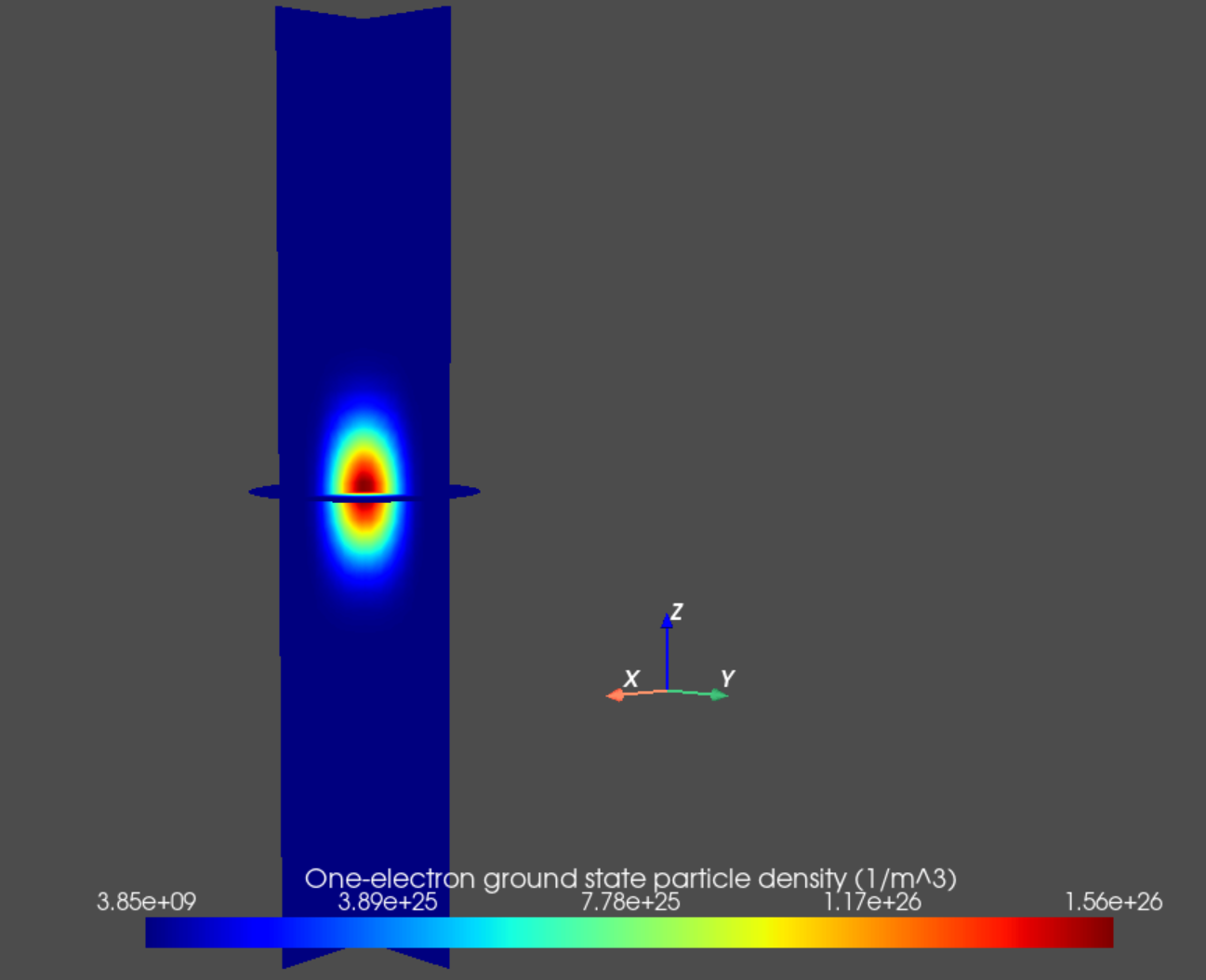
Fig. 14.5.1 One-electron ground state particle density
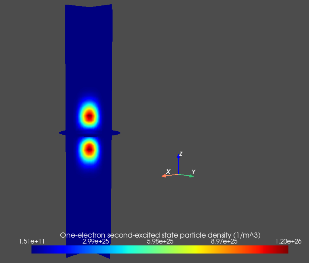
Fig. 14.5.2 One-electron second excited state particle density
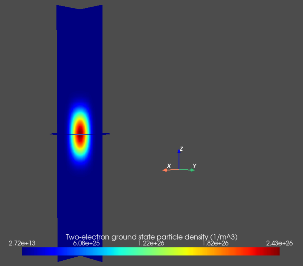
Fig. 14.5.3 Two-electron ground state particle density
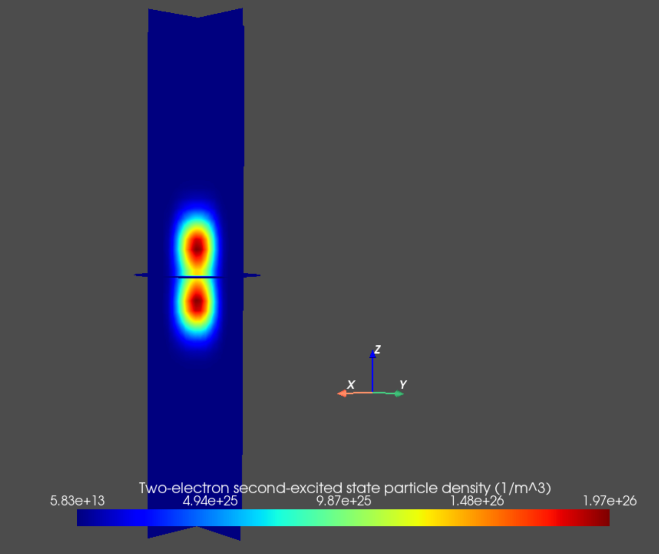
Fig. 14.5.4 Two-electron second excited state particle density
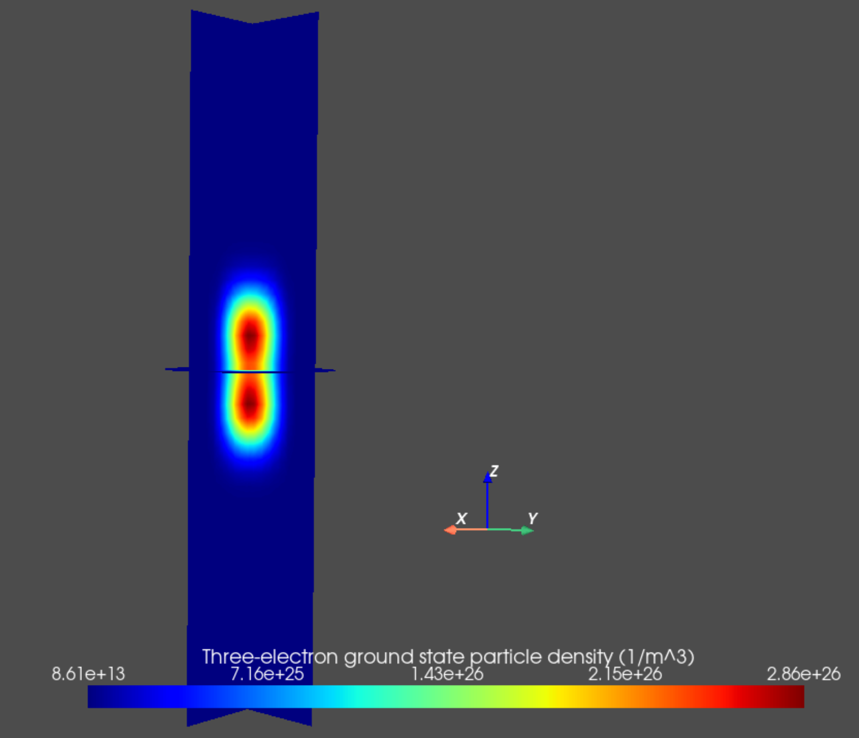
Fig. 14.5.5 Three-electron ground state particle density
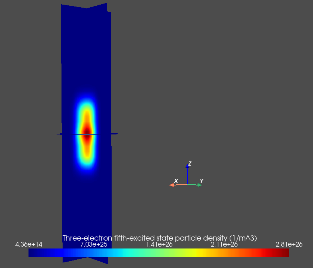
Fig. 14.5.6 Three-electron fifth excited state particle density
Note
The
Subspace objects stored in the
many_body_subspaces
of a
Device object account for
single-particle state degeneracy explicitly. As a result, in this example,
the particle density of the first single-electron “excited” state is the
same as for the single-electron ground state, simply because these states
are taken to be degenerate. Therefore, the first single-electron eigenstate
whose particle density differs from the ground state is the one with
eigenstate label \(2\).
14.6. Full code
__copyright__ = "Copyright 2022-2026, Nanoacademic Technologies Inc."

from qtcad.device import constants as ct
from qtcad.device.mesh3d import Mesh
from qtcad.device import io
from qtcad.device import analysis as an
from qtcad.device import materials as mt
from qtcad.device import Device
from qtcad.device.schrodinger import Solver as SingleBodySolver
import pathlib
from qtcad.device.many_body import Solver as ManyBodySolver
from qtcad.device.many_body import SolverParams

# Define some device parameters
Vgs = 0.5  # Gate-source bias
Ew = mt.Si.chi + mt.Si.Eg / 2  # Metal work function
Ltot = 20e-9  # Device height in m
radius = 2.5e-9  # Device radius in m

# Paths to mesh file and output files
script_dir = pathlib.Path(__file__).parent.resolve()
path_mesh = script_dir / "meshes/" / "nanowire.msh"
path_hdf5 = script_dir / "output/" / "nanowire.hdf5"

# Load the mesh
scaling = 1e-9
mesh = Mesh(scaling, str(path_mesh))

# Create device from mesh and set statistics.
# It is important to set statistics before creating boundaries since
# they determine the boundary values, Failing to do so will produce
# inconsistent results.
dvc = Device(mesh, conf_carriers="e")
dvc.statistics = "FD_approx"  # Analytic approximation to Fermi-Dirac statistics

# Create regions first.
# Make sure each element is assigned to a region, otherwise default
# (silicon) parameters are used
dvc.new_region("channel_ox", mt.SiO2)
dvc.new_region("source_ox", mt.SiO2)
dvc.new_region("drain_ox", mt.SiO2)
dvc.new_region("channel", mt.Si)
dvc.new_region("source", mt.Si, pdoping=5e20 * 1e6, ndoping=0)
dvc.new_region("drain", mt.Si, pdoping=5e20 * 1e6, ndoping=0)

# Then create boundaries
dvc.new_ohmic_bnd("source_bnd")
dvc.new_ohmic_bnd("drain_bnd")
dvc.new_gate_bnd("gate_bnd", Vgs, Ew)

# Load the electic potential
dvc.set_potential(io.load(path_hdf5, "phi"))

# Solve the single-electron problem
slv = SingleBodySolver(dvc)
slv.solve()
dvc.print_energies()

# Solve the many-body problem
solver_params = SolverParams()
solver_params.num_states = 3
solver_params.n_degen = 2
solver_params.alpha = 0.5
solver_params.num_particles = [0, 1, 2, 3]
slv = ManyBodySolver(dvc, solver_params=solver_params)
slv.solve()

# Many-body subspace properties
print("Many-body subspaces:", dvc.many_body_subspaces)
print("Number of subspaces:", len(dvc.many_body_subspaces))
print("Electron number in subspace 2:", dvc.many_body_subspaces[2].N)

print("Two-electron many-body basis set (integers): ")
print(dvc.get_N_particle_subspace(2).get_bas_set())

print("Two-electron many-body basis set (binary strings): ")
print(dvc.get_N_particle_subspace(2).get_bas_set(dtype="str"))

print("Two-electron many-body basis set (array): ")
print(dvc.get_N_particle_subspace(2).get_bas_set(dtype="array"))

print("Two-electron many-body eigenvalues (eV): ")
print(dvc.get_N_particle_subspace(2).eigval / ct.e)

print("Two-electron many-body ground state:")
print(dvc.get_N_particle_subspace(2).eigvec[:, 0])
print("Two-electron many-body first excited state:")
print(dvc.get_N_particle_subspace(2).eigvec[:, 1])

print("One-electron many-body basis set:")
print(dvc.get_N_particle_subspace(1).get_bas_set(dtype="array"))
print("One-electron many-body eigenstates:")
print(dvc.get_N_particle_subspace(1).eigvec)

# Many-body state objects
print("Two-electron ground-state coefficients and energy (eV)")
print(dvc.get_N_particle_subspace(2).get_eig_state(0).coeff)
print(dvc.get_N_particle_subspace(2).get_eig_state(0).energy / ct.e)

# Chemical potentials and Coulomb peak positions
print("Chemical potentials (eV)")
print(dvc.chem_potentials / ct.e)
print("Coulomb peak positions (V)")
print(dvc.coulomb_peak_pos)

# Plot electron density
an.plot_slices(
    mesh,
    dvc.get_many_body_density(1, 0),
    title="One-electron ground state particle density (1/m^3)",
)
an.plot_slices(
    mesh,
    dvc.get_many_body_density(1, 2),
    title="One-electron second-excited state particle density (1/m^3)",
)
an.plot_slices(
    mesh,
    dvc.get_many_body_density(2, 0),
    title="Two-electron ground state particle density (1/m^3)",
)
an.plot_slices(
    mesh,
    dvc.get_many_body_density(2, 2),
    title="Two-electron second-excited state particle density (1/m^3)",
)
an.plot_slices(
    mesh,
    dvc.get_many_body_density(3, 0),
    title="Three-electron ground state particle density (1/m^3)",
)
an.plot_slices(
    mesh,
    dvc.get_many_body_density(3, 5),
    title="Three-electron fifth-excited state particle density (1/m^3)",
)