18. Exchange coupling in a double quantum dot in FD-SOI—Part 1: Perturbation theory
18.1. Requirements
18.1.1. Software components
QTCAD
Gmsh
18.1.2. Geometry file
qtcad/examples/tutorials/meshes/dqdfdsoi.geo
18.1.3. Python script
qtcad/examples/tutorials/exchange_1.py
18.1.4. References
18.2. Briefing
In this tutorial, we will calculate the exchange interaction strength for a double quantum dot in the generic fully-depleted silicon-on-insulator (FD-SOI) geometry presented in A double quantum dot device in a fully-depleted silicon-on-insulator transistor. Here, we use the perturbation theory presented in Perturbation theory of exchange coupling in a double quantum dot to quickly evaluate the exchange interaction strength without requiring the costly exact diagonalization approach which will be presented in the next tutorial.
As explained in Perturbation theory of exchange coupling in a double quantum dot, in the symmetric configuration, the exchange interaction strength may be estimated within perturbation theory using only two quantities that are easily accessible through single-electron calculations: the tunnel coupling strength \(\Omega\) and the on-site Coulomb interaction energy \(U\). While the tunnel coupling strength was already considered in previous tutorials, here, we will evaluate the on-site Coulomb interaction energy. This will enable us to compute an estimate for the exchange interaction that we will later compare with an exact diagonalization calculation.
18.3. Header
We start by importing the necessary packages, classes, and functions.
import numpy as np
import pathlib
from qtcad.device import constants as ct
from qtcad.device import io
from qtcad.device.mesh3d import Mesh, SubMesh
from qtcad.device import SubDevice
from qtcad.device.poisson import SolverParams as PoissonSolverParams
from qtcad.device.poisson import Solver as PoissonSolver
from qtcad.device.schrodinger import SolverParams as SchrodingerSolverParams
from qtcad.device.schrodinger import Solver as SchrodingerSolver
from qtcad.device.many_body import Solver as ManyBodySolver
from qtcad.device.many_body import SolverParams as ManyBodySolverParams
from helper.double_dot_fdsoi import get_double_dot_fdsoi
These packages, classes, and functions were all seen in previous tutorials.
18.4. Setting up the device
As in Tunnel coupling in a double quantum dot in FD-SOI—Part 1: Plunger gate tuning, we will set up the device using the
get_double_dot_fdsoi function defined in A double quantum dot device in a fully-depleted silicon-on-insulator transistor.
We first set up paths for the mesh file and for output files.
# Set up paths
script_dir = pathlib.Path(__file__).parent.resolve()
# mesh path
path_mesh = script_dir / "meshes"
path_out = script_dir / "output"
We then load the strongest tunnel coupling that was calculated in Tunnel coupling in a double quantum dot in FD-SOI—Part 2: Tuning the barrier gate and saved into a text file.
# Load the tunnel coupling from strong-tunneling simulation
path_tunnel = path_out / "tunnel_coupling_low_barrier.txt"
tunnel_coupling = np.loadtxt(path_tunnel)
This tunnel coupling is one of the two parameters required to calculate exchange within the perturbation theory explained in Perturbation theory of exchange coupling in a double quantum dot. In the rest of this tutorial, we will thus focus on calculating the on-site Coulomb interaction \(U\).
The next step is to load the mesh. To expedite convergence of the non-linear Poisson solver, we load the mesh that was already obtained in Tunnel coupling in a double quantum dot in FD-SOI—Part 1: Plunger gate tuning thanks to adaptive refinement.
# Load the mesh
scaling = 1e-9
path_file = str(path_mesh / "refined_dqdfdsoi.msh")
mesh = Mesh(scaling, path_file)
We then set the gate biases. Here, instead of aiming at a symmetric configuration, we introduce a detuning between the plunger gates that is large enough to ensure that the first two single-electron eigenstates of the double dot are localized in the left and right dots, but still too small to distort the confinement potential in a way that would lead to Coulomb integrals that are not representative of the localized left and right states. After some trial and error, we find that a detuning of \(5~\textrm{meV}\) is adequate.
# Define the gate biases
detuning = 5e-3
back_gate_bias = -0.5
barrier_gate_1_bias = 0.5
plunger_gate_1_bias = 0.59
barrier_gate_2_bias = 0.57
plunger_gate_2_bias = 0.59 + detuning
barrier_gate_3_bias = 0.5
We then define the device and create a submesh object for the double quantum dot region.
# Define the device
dvc = get_double_dot_fdsoi(mesh, back_gate_bias, barrier_gate_1_bias,
    plunger_gate_1_bias, barrier_gate_2_bias, plunger_gate_2_bias,
    barrier_gate_3_bias)

# List of regions forming the double quantum dot region
dot_region_list = ["oxide_dot", "gate_oxide_dot", "buried_oxide_dot",
                    "channel_dot"]

# Create the submesh object for the dot region
submesh = SubMesh(dvc.mesh, dot_region_list)
18.5. Basic electrostatics and eigenstates in a localized configuration
Since the gate bias configuration is still close to the one employed in Tunnel coupling in a double quantum dot in FD-SOI—Part 1: Plunger gate tuning, we start by loading the final electric potential that was saved after solving non-linear Poisson in that previous run.
# Load the electric potential from the previous run to speed up Poisson
# calculation
phi = io.load(path_out / "tunnel_coupling_final_potential.hdf5",
    var_name="phi")
dvc.set_potential(phi)
Using this potential as an initial guess will help speed up convergence of
the non-linear Poisson
Solver.
We configure the non-linear Poisson and Schrödinger solver parameters with
# Configure the non-linear Poisson solver
params_poisson = PoissonSolverParams()
params_poisson.tol = 1e-3 # Convergence threshold (tolerance) for the error

# Configure the Schrödinger solver
params_schrod = SchrodingerSolverParams()
params_schrod.tol = 1e-6      # Tolerance on energies in eV
We then instantiate the Poissson Solver
and run its solve method with
the initialize argument set to False to use the potential
that is already stored in the
Device object as an initial guess.
We also save the potential in a file for later use.
# Instantiate Poisson solver
poisson_slv = PoissonSolver(dvc, solver_params=params_poisson)

# Solve Poisson's equation
poisson_slv.solve(initialize=False)

# Save the potential
path_potential = path_out / "detuned_potential.hdf5"
io.save(path_potential, dvc.phi, var_name="phi")
We then set the confinement potential from the solution of the non-linear
Poisson equation, create a SubDevice
object for the double quantum dot region, instantiate a Schrödinger
Solver, run it, print the
resulting single-electron eigenenergies, and save the ground and first
excited state wavefunctions.
# Get the potential energy from the band edge for usage in the Schrodinger
# solver
dvc.set_V_from_phi()

# Create a subdevice for the dot region
subdvc = SubDevice(dvc, submesh)

# Create a Schrodinger solver, and run it
schrod_solver = SchrodingerSolver(subdvc, solver_params=params_schrod)
schrod_solver.solve()
subdvc.print_energies()

# Save the ground and first excited state wavefunctions into .vtu files
path_states = path_out / "exchange_localized_wavefunctions.vtu"
out_dict = {
    "Ground state": subdvc.eigenfunctions[:,0],
    "First excited state": subdvc.eigenfunctions[:,1]
}
io.save(path_states, out_dict, submesh)
Plotting the wavefunctions in ParaView, we find that the ground and first excited states are well localized in the right and left dots, respectively.
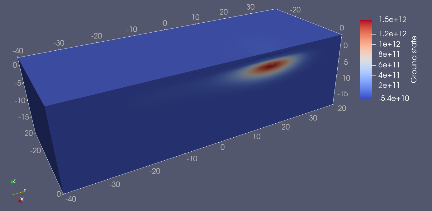
Fig. 18.5.1 Double quantum dot ground state.
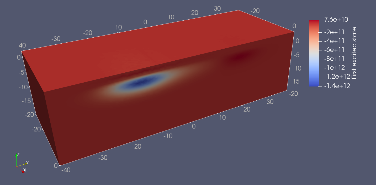
Fig. 18.5.2 Double quantum dot first excited state.
18.6. Coulomb integrals
Now that well-localized single-electron states have been found, we may readily calculate their Coulomb integrals to evaluate the on-site Coulomb interaction.
To do so, we instantiate a many-body
Solver object.
# Instantiate a many-body solver
manybody_solver_params = ManyBodySolverParams()
manybody_solver_params.num_states = 2
manybody_solver_params.overlap = False
manybody_solver = ManyBodySolver(subdvc, solver_params=manybody_solver_params)
We set num_states to 2, because we are only interested in the Coulomb
integrals matrix in the basis spanned by the localized left and right states of
the double quantum dot. In addition, we set overlap to False, because
we are not interested in overlap integrals such as \(V_\mathrm{LRRL}\).
We then compute the Coulomb integrals matrix, print it, and save it in a text file.
# Compute the matrix of Coulomb integrals
coulomb_mat = manybody_solver.get_coulomb_matrix(overlap = False)
print('Coulomb interaction matrix in a nearly localized single-electron basis set')
print(coulomb_mat[0:2,0:2]/ct.e)

# Export the coulomb matrix
np.savetxt(path_out/"exchange_coulomb_localized.txt", coulomb_mat)
We obtain the following results.
Coulomb interaction matrix in a nearly localized single-electron basis set
[[0.01723048 0.00406259]
[0.00406259 0.0168071 ]]
Knowing from the above analysis that the ground state is localized in the right dot (corresponding to \(|\mathrm R\rangle\)), and that the first excited state is localized in the left dot (corresponding to \(|\mathrm L\rangle\)), we may associate this matrix with
Therefore, we have found \(V_L \approx 16.8~\textrm{meV}\), \(V_R \approx 17.2~\textrm{meV}\), and \(V_\mathrm{LR} = V_\mathrm{RL} \approx 4.1~\textrm{meV}\).
We remark that the inter-site Coulomb interaction, while significant, is a factor of four smaller than the on-site Coulomb interaction, and may thus be neglected in a first approximation, when interest mostly lies in the order of magnitude of the exchange interaction strength. In addition, the asymmetric bias used here to localize the eigenstates has introduced a small difference (\(\approx 0.5~\textrm{meV}\)) between \(V_\mathrm L\) and \(V_\mathrm R\) which we will neglect here.
18.7. Exchange interaction strength
Knowing both the tunnel coupling and Coulomb interaction strengths, we are ready to evaluate the exchange interaction strength using Eq. (9.8).
# Calculate the theoretical exchange coupling
exchange = (tunnel_coupling*ct.e)**2 / coulomb_mat[0,0]
print("Theoretical exchange interaction: {:.3f} MHz".format(exchange/ct.h/1e6))

# Export the theoretical exchange coupling
np.savetxt(path_out/"exchange_perturbation.txt", np.array([exchange]))
In addition to printing the value of the exchange interaction strength, we save it in a text file (in SI units) for further use in the next tutorial.
Expressing the exchange interaction strength in MHz, we find
Theoretical exchange interaction: 929.216 MHz
In the next tutorial, Exchange coupling in a double quantum dot in FD-SOI—Part 2: Exact diagonalization, we will compare this value with the output of an exact diagonalization approach.
18.8. Full code
__copyright__ = "Copyright 2022-2026, Nanoacademic Technologies Inc."

import numpy as np
import pathlib
from qtcad.device import constants as ct
from qtcad.device import io
from qtcad.device.mesh3d import Mesh, SubMesh
from qtcad.device import SubDevice
from qtcad.device.poisson import SolverParams as PoissonSolverParams
from qtcad.device.poisson import Solver as PoissonSolver
from qtcad.device.schrodinger import SolverParams as SchrodingerSolverParams
from qtcad.device.schrodinger import Solver as SchrodingerSolver
from qtcad.device.many_body import Solver as ManyBodySolver
from qtcad.device.many_body import SolverParams as ManyBodySolverParams
from helper.double_dot_fdsoi import get_double_dot_fdsoi

# Set up paths
script_dir = pathlib.Path(__file__).parent.resolve()
# mesh path
path_mesh = script_dir / "meshes"
path_out = script_dir / "output"

# Load the tunnel coupling from strong-tunneling simulation
path_tunnel = path_out / "tunnel_coupling_low_barrier.txt"
tunnel_coupling = np.loadtxt(path_tunnel)

# Load the mesh
scaling = 1e-9
path_file = str(path_mesh / "refined_dqdfdsoi.msh")
mesh = Mesh(scaling, path_file)

# Define the gate biases
detuning = 5e-3
back_gate_bias = -0.5
barrier_gate_1_bias = 0.5
plunger_gate_1_bias = 0.59
barrier_gate_2_bias = 0.57
plunger_gate_2_bias = 0.59 + detuning
barrier_gate_3_bias = 0.5

# Define the device
dvc = get_double_dot_fdsoi(
    mesh,
    back_gate_bias,
    barrier_gate_1_bias,
    plunger_gate_1_bias,
    barrier_gate_2_bias,
    plunger_gate_2_bias,
    barrier_gate_3_bias,
)

# List of regions forming the double quantum dot region
dot_region_list = ["oxide_dot", "gate_oxide_dot", "buried_oxide_dot", "channel_dot"]

# Create the submesh object for the dot region
submesh = SubMesh(dvc.mesh, dot_region_list)

# Load the electric potential from the previous run to speed up Poisson
# calculation
phi = io.load(path_out / "tunnel_coupling_final_potential.hdf5", var_name="phi")
dvc.set_potential(phi)

# Configure the non-linear Poisson solver
params_poisson = PoissonSolverParams()
params_poisson.tol = 1e-3  # Convergence threshold (tolerance) for the error

# Configure the Schrödinger solver
params_schrod = SchrodingerSolverParams()
params_schrod.tol = 1e-6  # Tolerance on energies in eV

# Instantiate Poisson solver
poisson_slv = PoissonSolver(dvc, solver_params=params_poisson)

# Solve Poisson's equation
poisson_slv.solve(initialize=False)

# Save the potential
path_potential = path_out / "detuned_potential.hdf5"
io.save(path_potential, dvc.phi, var_name="phi")

# Get the potential energy from the band edge for usage in the Schrodinger
# solver
dvc.set_V_from_phi()

# Create a subdevice for the dot region
subdvc = SubDevice(dvc, submesh)

# Create a Schrodinger solver, and run it
schrod_solver = SchrodingerSolver(subdvc, solver_params=params_schrod)
schrod_solver.solve()
subdvc.print_energies()

# Save the ground and first excited state wavefunctions into .vtu files
path_states = path_out / "exchange_localized_wavefunctions.vtu"
out_dict = {
    "Ground state": subdvc.eigenfunctions[:, 0],
    "First excited state": subdvc.eigenfunctions[:, 1],
}
io.save(path_states, out_dict, submesh)

# Instantiate a many-body solver
manybody_solver_params = ManyBodySolverParams()
manybody_solver_params.num_states = 2
manybody_solver_params.overlap = False
manybody_solver = ManyBodySolver(subdvc, solver_params=manybody_solver_params)

# Compute the matrix of Coulomb integrals
coulomb_mat = manybody_solver.get_coulomb_matrix(overlap=False)
print("Coulomb interaction matrix in a nearly localized single-electron basis set")
print(coulomb_mat[0:2, 0:2] / ct.e)

# Export the coulomb matrix
np.savetxt(path_out / "exchange_coulomb_localized.txt", coulomb_mat)

# Calculate the theoretical exchange coupling
exchange = (tunnel_coupling * ct.e) ** 2 / coulomb_mat[0, 0]
print("Theoretical exchange interaction: {:.3f} MHz".format(exchange / ct.h / 1e6))

# Export the theoretical exchange coupling
np.savetxt(path_out / "exchange_perturbation.txt", np.array([exchange]))