5. Schrödinger equation for a quantum dot

5.1. Requirements

5.1.1. Software components

• QTCAD

5.1.2. Python script

• qtcad/examples/tutorials/creating_dot.py

5.1.3. References

• Poisson and Schrödinger simulation of a GAAFET

5.2. Briefing

The aim of this tutorial is to demonstrate how QTCAD can be used to solve the Schrödinger equation for a quantum-dot system.

5.3. Setting up the device

5.3.1. Header

In addition to what has already been invoked in gaafet.py (see the previous tutorial), here we also need to import the SubMesh and SubDevice classes which will enable us to find states confined to a specific region of space, e.g. a quantum dot.

import numpy as np
from matplotlib import pyplot as plt
import pathlib

from device.mesh3d import Mesh, SubMesh
from device import constants as ct
from device.analysis import linecut
from device import io

from device import materials as mt
from device import Device, SubDevice
from device.schrodinger import Solver, SolverParams

5.3.2. Load data and device setup

In this tutorial, we will construct an artificial example for illustrative purposes. The example we are considering is a rectangular prism where the \(x\) dimension is split into 5 parts: 2 lead regions, 2 barrier regions, and a dot region. The barriers are between the leads and the dot on either side of the dot (along the \(x\) direction). These different regions have been tagged using Gmsh (see qtcad/examples/tutorials/meshes/lead_dot_lead.geo). We start by loading the appropriate mesh and defining paths for output files.

# Paths to mesh file and output files
script_dir = pathlib.Path(__file__).parent.resolve()
path_mesh = script_dir / "meshes" / "lead_dot_lead.msh2"
path_V = script_dir / "output" / "creating_dot_V.vtu"
path_psi0 = script_dir / "output" / "creating_dot_psi0.vtu"
path_psi1 = script_dir / "output" / "creating_dot_psi1.vtu"

# Load and plot the mesh
scalingFactor = 1e-9
mesh = Mesh(scalingFactor, str(path_mesh))
mesh.show()

The mesh is shown below.

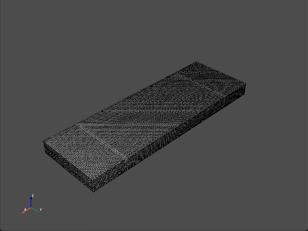
Fig. 5.3.1 Quantum dot mesh

From the mesh we then create a device.

# Create the device from the mesh
d = Device(mesh, conf_carriers="e")

d.new_region('dot', mt.GaAs)
d.new_region('lead', mt.GaAs)
d.new_region('lead2', mt.GaAs)
d.new_region('barrier', mt.GaAs)
d.new_region('barrier2', mt.GaAs)

We have specified that the five regions that make up the entire device will be made from GaAs.

5.3.3. Defining the potential

Next, we define the potential along the \(y\) and \(z\) directions

# Potential along y and z
# Position of the harmonic oscillator minimum
y0 = 0
z0 = 0
Ky = 2e-7 # Parabolic in y
Kz = 1e-4 # Parabolic in z

def V_func(x,y,z):
   Vy = Ky/2.*(y-y0)**2
   Vz = Kz/2. * (z-z0)**2
   return Vy + Vz

# Set the potential energy
d.set_V(V_func)

The setter for the potential set_V fixes the quadratic potential along y and z in the device.

To define the potential along x, we use the add_to_V method which allows us to add a constant potential to different regions of space. The first input is the potential to be added and the key-word argument region specifies for which region the V is to be added to the potential:

# Add the potential energy along x
d.add_to_V(12e-3 * ct.e, region='barrier')
d.add_to_V(12e-3 * ct.e, region='barrier2')
d.add_to_V(-10e-3 * ct.e, region='lead')
d.add_to_V(-10e-3 * ct.e, region='lead2')
d.add_to_V(-1e-2 * ct.e)

If no region is specified, V is added to all regions. Using this method we construct a potential with 2 barriers, separating a central “dot” from 2 leads. Plots of the potential are shown below.

Note that if we were to first apply the Poisson solver to the device, we could get the potential corresponding to the band edges by using the device method set_V_from_phi(). This method is useful if, for example, the goal was to study the effect of a perturbing potential in addition to the one generated from the Poisson solver. In this case, one could apply the Poisson solver and then run

d.set_V_from_phi()
d.set_V(d.V + V)

where d is the device under consideration and V is the perturbing potential one intends to add. We would then be able to follow the steps below.

5.4. Creating the dot

Now that the device has been set up, we create a dot region to solve for the quantum dot eigenstates. We start by identifying which regions will be included in the dot’s mesh. In this case, we will include the regions tagged, using Gmsh, as 'dot', 'barrier', and 'barrier2'. The barriers must be included in the dot’s mesh because they provide the confinement for the electrons bound to the dot. We create SubMesh over for the dot region using:

# Create submesh
dotmesh = SubMesh(d.mesh, ['dot', 'barrier', 'barrier2'])

The SubMesh constructor takes 2 inputs, the mesh we are creating a submesh from and a list of tags of the regions to be included in the submesh. In this case the parent mesh is that of the full device, stored in d.mesh. From here we can create a SubDevice using

# Create subdevice
dot = SubDevice(d, dotmesh)

This constructor takes as input the full (parent) device and the submesh from which we wish to construct our subdevice. Now dot is a device and has all the associated attributes and methods. In particular, we can apply the Schrödinger solver to solve for the eigenstates of the dot device:

# Solve the Schrodinger equation.
# # Configure the Schrödinger solver
params_schrod = SolverParams()
params_schrod.num_states = 3 # Number of energy levels to consider
params_schrod.tol = 1e-9 # Set the tolerance for convergence

# # Create solver
s = Solver(dot, solver_params=params_schrod)
s.solve() # solve

In the first line, we instantiate a SolverParams object appropriate for Schrödinger solvers. The second specifies the number of eigenstates and energies to consider in the diagonalization of the dot Hamiltonian. Line 3 sets the tolerance for convergence on energies in electron-volts. Then, the solver is created with the appropriated parameters and the solve method is run to solve the Schrödinger equation for the dot. Note the confinement potential is located in the attribute dot.V.

5.5. Eigenenergies and eigenfunctions

We can print the eigenenergies using the print_energies() method:

dot.print_energies()

which outputs the eigenergies in eV units.

Energy levels (eV)
[-0.00018985  0.00018604  0.00081295]

Finally, we can use the linecut function to get linecuts of the potential and wavefunctions and plot them. We start of getting the global nodes of the dotmesh:

# Global nodes in dot region
xdot = dotmesh.glob_nodes[:, 0]
ydot = dotmesh.glob_nodes[:, 1]
zdot = dotmesh.glob_nodes[:, 2]

Then, we create the beginning and end points for a linecut along x. For the dot wavefunction, we choose to fix the y and z coordinates at 0, and take the linecut from the minimal to maximal x coordinate. A similar approach is applied for the linecut of the potential except instead of the minimal and maximal x values of the dotmesh, we use the minimal and maximal x values of the full device mesh, mesh, because the potential is defined on the entire device.

# Global nodes in full device
x = mesh.glob_nodes[:, 0]
y = mesh.glob_nodes[:, 1]
z = mesh.glob_nodes[:, 2]

# Linecut coordinates for wave function and potential energy
beginwf = (np.min(xdot), y0, z0); endwf = (np.max(xdot), y0, z0)
beginV = (np.min(x), y0, z0); endV = (np.max(x), y0, z0)

Next we apply the linecut function to generate the linecuts

# Linecuts of ground state squared and potential energy
psiposx, psix0 = linecut(dotmesh, np.abs(dot.eigenfunctions[:, 0])**2,
   beginwf, endwf)
psiposx += np.min(xdot)
Vposx, Vx = linecut(mesh, d.V, beginV, endV)
Vposx += np.min(x)

The linecut function takes as inputs the appropriate mesh, the quantity we wish to evaluate along the linecut and the beginning and end points of the linecut. The outputs are the distance along the linecut (starting at 0) and the quantity of interest along the line from the beginning to the end point. Here we add the minimal x values to the positions to convert the distance along the linecut to an x coordinate. An identical approach is applied for the linecut along y:

beginy = ((np.max(x) + np.min(x))/2, np.min(y), z0)
endy = ((np.max(x) + np.min(x))/2, np.max(y), z0)
psiposy, psiy0 = linecut(dotmesh, np.abs(dot.eigenfunctions[:, 0])**2,
   beginy, endy)
psiposy += np.min(ydot)
Vposy, Vy = linecut(mesh, d.V, beginy, endy)
Vposy += np.min(y)

We then plot these linecuts using the following code.

nm = 1e-9

# Plotting eigenstates along x
fig, ax1 = plt.subplots()
ax1.set_title('Linecut along x')
ax1.plot(psiposx / nm, psix0)
ax2 = ax1.twinx()
ax2.plot(Vposx / nm, Vx / ct.e, '--')
ax1.grid()
ax1.set_xlabel("x (nm)")
ax1.set_ylabel(r"$|\Psi(x, y_0, z_0)|^2 (1/m^3)$")
ax2.set_ylabel(r"$V (eV)$")

# Display
plt.tight_layout()
plt.show()

# Plotting eigenstates along y
fig, ax3 = plt.subplots()
ax3.set_title('Linecut along y')
ax3.plot(psiposy / nm, psiy0)
ax4 = ax3.twinx()
ax4.plot(Vposy / nm, Vy / ct.e, '--')
ax3.grid()
ax3.set_xlabel("y (nm)")
ax3.set_ylabel(r"$|\Psi(x_0 , y, z_0)|^2 (1/m^3)$")
ax4.set_ylabel(r"$V (eV)$")

# Display
plt.tight_layout()
plt.show()

This produces the figure shown below.

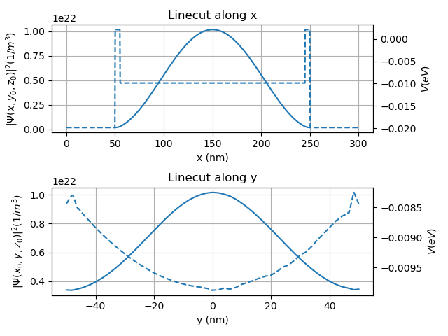
Fig. 5.5.1 Linecuts of the potential (dotted line) and ground state (solid line)

5.6. Saving relevant quantities

We can also save relevant quantities such as the potential and the ground and first excited wavefunctions in .vtu format to be visualized later. We pass the path, the array to save, and the mesh to the io.save method which will decipher what type of file to save the array as from the extension used in the file path.

# Saving in .vtu format
io.save(str(path_V), d.V, mesh)
io.save(str(path_psi0),
        dot.eigenfunctions[:,0],
        dotmesh
        )
io.save(str(path_psi1),
        dot.eigenfunctions[:,1],
        dotmesh
        )

In Visualizing QTCAD quantities with ParaView we will see how to use ParaView to visualize these outputs.

5.7. Full code

__copyright__ = "Copyright 2023, Nanoacademic Technologies Inc."

import numpy as np
from matplotlib import pyplot as plt
import pathlib
from device.mesh3d import Mesh, SubMesh
from device import constants as ct
from device.analysis import linecut
from device import io
from device import materials as mt
from device import Device, SubDevice
from device.schrodinger import Solver, SolverParams

# Paths to mesh file and output files
script_dir = pathlib.Path(__file__).parent.resolve()
path_mesh = script_dir / "meshes" / "lead_dot_lead.msh2"
path_V = script_dir / "output" / "creating_dot_V.vtu"
path_psi0 = script_dir / "output" / "creating_dot_psi0.vtu"
path_psi1 = script_dir / "output" / "creating_dot_psi1.vtu"

# Load and plot the mesh
scalingFactor = 1e-9
mesh = Mesh(scalingFactor, str(path_mesh))
mesh.show()

# Create the device from the mesh
d = Device(mesh, conf_carriers="e")

d.new_region('dot', mt.GaAs)
d.new_region('lead', mt.GaAs)
d.new_region('lead2', mt.GaAs)
d.new_region('barrier', mt.GaAs)
d.new_region('barrier2', mt.GaAs)

# Potential along y and z
# Position of the harmonic oscillator minimum
y0 = 0 
z0 = 0
Ky = 2e-7 # Parabolic in y
Kz = 1e-4 # Parabolic in z

def V_func(x,y,z):
   Vy = Ky/2.*(y-y0)**2
   Vz = Kz/2. * (z-z0)**2
   return Vy + Vz

# Set the potential energy
d.set_V(V_func)

# Add the potential energy along x
d.add_to_V(12e-3 * ct.e, region='barrier')
d.add_to_V(12e-3 * ct.e, region='barrier2')
d.add_to_V(-10e-3 * ct.e, region='lead')
d.add_to_V(-10e-3 * ct.e, region='lead2')
d.add_to_V(-1e-2 * ct.e)

# Create submesh
dotmesh = SubMesh(d.mesh, ['dot', 'barrier', 'barrier2'])

# Create subdevice
dot = SubDevice(d, dotmesh)

# Solve the Schrodinger equation.
# # Configure the Schrödinger solver
params_schrod = SolverParams()
params_schrod.num_states = 3 # Number of energy levels to consider
params_schrod.tol = 1e-9 # Set the tolerance for convergence

# # Create solver
s = Solver(dot, solver_params=params_schrod)
s.solve() # solve

dot.print_energies()

# Global nodes in dot region
xdot = dotmesh.glob_nodes[:, 0]
ydot = dotmesh.glob_nodes[:, 1]
zdot = dotmesh.glob_nodes[:, 2] 

# Global nodes in full device
x = mesh.glob_nodes[:, 0]
y = mesh.glob_nodes[:, 1]
z = mesh.glob_nodes[:, 2]

# Linecut coordinates for wave function and potential energy
beginwf = (np.min(xdot), y0, z0); endwf = (np.max(xdot), y0, z0)
beginV = (np.min(x), y0, z0); endV = (np.max(x), y0, z0)

# Linecuts of ground state squared and potential energy
psiposx, psix0 = linecut(dotmesh, np.abs(dot.eigenfunctions[:, 0])**2, 
   beginwf, endwf)
psiposx += np.min(xdot)
Vposx, Vx = linecut(mesh, d.V, beginV, endV)
Vposx += np.min(x)

beginy = ((np.max(x) + np.min(x))/2, np.min(y), z0)
endy = ((np.max(x) + np.min(x))/2, np.max(y), z0)
psiposy, psiy0 = linecut(dotmesh, np.abs(dot.eigenfunctions[:, 0])**2, 
   beginy, endy)
psiposy += np.min(ydot)
Vposy, Vy = linecut(mesh, d.V, beginy, endy)
Vposy += np.min(y)

nm = 1e-9

# Plotting eigenstates along x
fig, ax1 = plt.subplots()
ax1.set_title('Linecut along x')
ax1.plot(psiposx / nm, psix0)
ax2 = ax1.twinx()
ax2.plot(Vposx / nm, Vx / ct.e, '--')
ax1.grid()
ax1.set_xlabel("x (nm)")
ax1.set_ylabel(r"$|\Psi(x, y_0, z_0)|^2 (1/m^3)$")
ax2.set_ylabel(r"$V (eV)$")

# Display
plt.tight_layout()
plt.show()

# Plotting eigenstates along y
fig, ax3 = plt.subplots()
ax3.set_title('Linecut along y')
ax3.plot(psiposy / nm, psiy0)
ax4 = ax3.twinx()
ax4.plot(Vposy / nm, Vy / ct.e, '--')
ax3.grid()
ax3.set_xlabel("y (nm)")
ax3.set_ylabel(r"$|\Psi(x_0 , y, z_0)|^2 (1/m^3)$")
ax4.set_ylabel(r"$V (eV)$")

# Display
plt.tight_layout()
plt.show()

# Saving in .vtu format
io.save(str(path_V), d.V, mesh)
io.save(str(path_psi0),
        dot.eigenfunctions[:,0],
        dotmesh
        )
io.save(str(path_psi1),
        dot.eigenfunctions[:,1],
        dotmesh
        )