20. Point charges in a double quantum dot in FD-SOI
20.1. Requirements
20.1.1. Software components
QTCAD
Gmsh
20.1.2. Geometry file
qtcad/examples/tutorials/meshes/dqdfdsoi.geo
20.1.3. Python script
qtcad/examples/tutorials/fdsoi_point_charges.py
20.1.4. References
20.2. Briefing
In this tutorial, we will investigate the effect of a point charge on the orbital levels of a quantum dot in the fully-depleted silicon-on-insulator (FD-SOI) geometry introduced in A double quantum dot device in a fully-depleted silicon-on-insulator transistor. Specifically, we will investigate how the spectrum of a quantum dot changes as a function of the position of a point charge in the device. In QTCAD, point charges are handled in accordance with the theoretical formulation presented in Point Charges.
20.3. Geometry file
As before, the initial mesh is generated from a
geometry file qtcad/examples/tutorials/meshes/dqdfdsoi.geo
by running Gmsh with
gmsh dqdfdsoi.geo
As in Tunnel coupling in a double quantum dot in FD-SOI—Part 1: Plunger gate tuning, this will produce a .msh file and a
.xao file. The .xao file format is appropriate for
geometries produced using the OpenCASCADE geometry kernel.
20.4. Header
We start by importing the necessary packages, classes, and functions.
import numpy as np
import matplotlib.pyplot as plt
import pathlib
import os
from joblib import load

from qtcad.device.mesh3d import Mesh, SubMesh
from qtcad.device.device import Device, SubDevice
from qtcad.device.poisson import Solver, SolverParams
from qtcad.device.schrodinger import Solver as SchrodingerSolver
from qtcad.device.schrodinger import SolverParams as SchrodingerSolverParams
from qtcad.device import constants as ct

from helper.double_dot_fdsoi import get_double_dot_fdsoi
All of these packages, classes, and functions have been introduced in previous
tutorials.
There is one exception: the load function from the joblib package.
This function will be used to load the profile of the point charge that was
saved in the MVEMT applied to a donor in silicon tutorial and use it to model charge impurities.
20.5. Setting up the device
We start with setting up paths to various files, both inputs and outputs. The inputs include the mesh file, the raw geometry file, and the refined mesh file. We also have the path to the profile generated via the MVEMT applied to a donor in silicon tutorial. The outputs are: two files that will contain the energy levels of the double-dot system as a function of the point charge position and two files containing a plot of the orbital level spacing as a function of the point-charge position. The difference between the two sets of files is that one will contain the results using a Gaussian profile for the point charge and the other will contain the results using a profile that is loaded from the MVEMT applied to a donor in silicon tutorial (which modeled a phosphorus donor in silicon).
# Files -----------------------------------------------------------------------
script_dir           = pathlib.Path(__file__).parent.resolve()

path_mesh            = script_dir / "meshes"
path_out             = script_dir / "output"

mesh_file            = str(path_mesh / "dqdfdsoi.msh")
geo_file             = str(path_mesh / "dqdfdsoi.xao")
ref_file             = str(path_mesh / "refined_dqdfdsoi_oxide.msh")
donor_profile_file   = str(path_out / "pc_density_profile_0.050_4.0.joblib")

E_file_G             = str(path_out / "fdsoi_energies_oxide_charge_G.txt")
Delta_file_G         = str(path_out / "DeltaE_oxide_G.png")
E_file_D             = str(path_out / "fdsoi_energies_oxide_charge_D.txt")
Delta_file_D         = str(path_out / "DeltaE_oxide_D.png")
We then setup the calculation by loading the mesh and defining the gate bias parameters.
# Setup -----------------------------------------------------------------------

# Load the mesh
scaling              = 1e-9
mesh                 = Mesh(scaling, mesh_file)

# Define the gate bias parameters
back_gate_bias       = -0.5
barrier_gate_1_bias  = 0.5
plunger_gate_1_bias  = 0.7
barrier_gate_2_bias  = 0.5
plunger_gate_2_bias  = 0.6
barrier_gate_3_bias  = 0.5
Here we have detuned the plunger-gate voltages such that the ground and first excited states of the system are localized under plunger gate 1 (see Fig. 20.5.1 and Fig. 20.5.2).
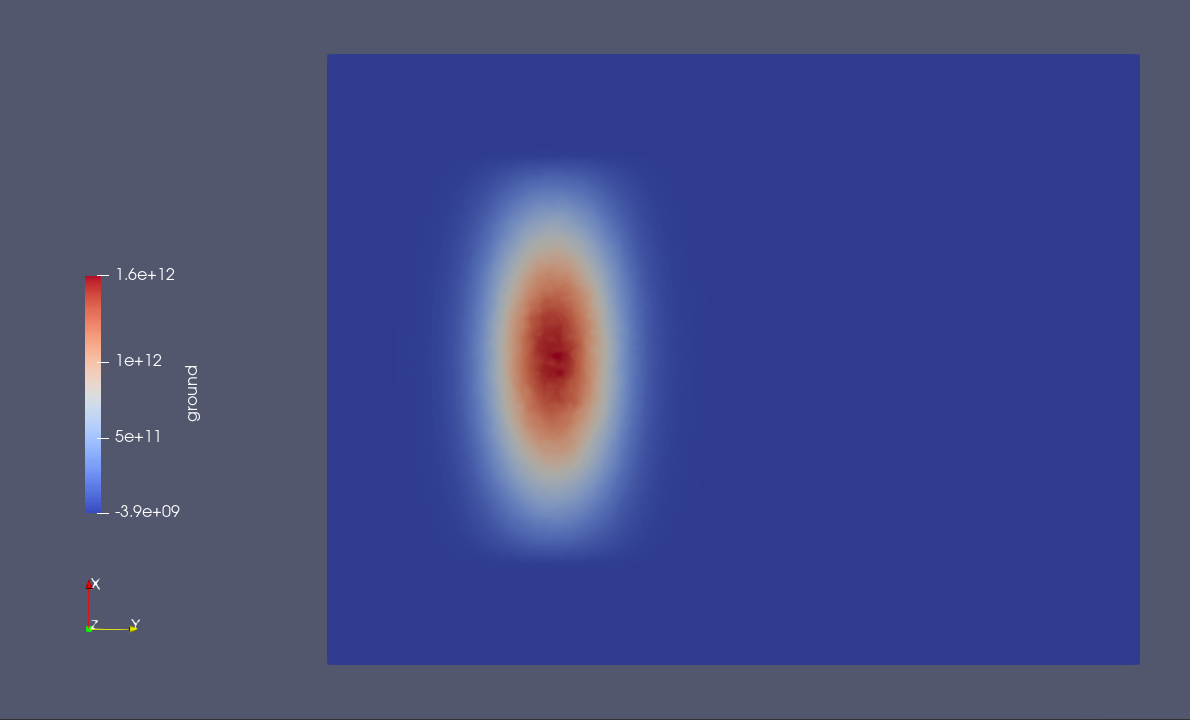
Fig. 20.5.1 Ground-state wavefunction localized under plunger gate 1.

Fig. 20.5.2 Excited-state wavefunction localized under plunger gate 1.
20.6. Basic electrostatics
Next, we create a function, func_poisson that can position point charges
throughout a double-dot FD-SOI device generated via the get_double_dot_fdsoi
function and apply the adaptive non-linear Poisson solver.
The inputs of func_poisson are the positions of the point charges, the
charges of each of the point charges, and the smearing radius of the point
charges.
There is also an optional argument, prof, that specifies the profile of the
point charges.
By default, the profile is Gaussian.
It returns the device over which the non-linear Poisson solver has been
applied.
The difference between this tutorial and previous ones is the use of the
add_point_charges method.
The arguments of this method are the positions of the point charges, the
charges of the point charges, the smearing radius of the point charges, and a
boolean that indicates whether the mesh should be refined around the point
charges (see Fig. 20.6.1).
This refinement is often necessary since the smearing radius is typically taken
to be smaller than the characteristic length of the mesh
elements
(\(\sigma \lesssim 0.1 \, \mathrm{nm} < 1 \, \mathrm{nm} \lesssim h\),
where \(\sigma\) is the smearing radius and \(h\) is a typical characteristic
length of a QTCAD mesh), which can lead to situations where the point charges
are not observed by the solvers.
# Poisson ---------------------------------------------------------------------
def func_poisson(pos: np.ndarray, Q: np.ndarray, r: float, prof='Gaussian') -> Device:
    """Apply the adaptive non-linear Poisson solver with point charges.
    Args:
        pos (np.ndarray): Position of the point charges
        Q (np.ndarray): Charge of the point charges
        r (float): Smearing radius of the point charges
        prof (str): Profile of the point charges
    Returns:
        device: Device over which the non-linear Poisson solver has been
            applied (point charges have been included).
    """

    # Define the device object from the function defined in the FD-SOI tutorial
    dvc = get_double_dot_fdsoi(mesh, back_gate_bias, barrier_gate_1_bias,
        plunger_gate_1_bias, barrier_gate_2_bias, plunger_gate_2_bias,
        barrier_gate_3_bias)

    dvc.add_point_charges(pos, Q, r=r, refine=True, profile=prof)

    # Configure the Non-Linear Poisson solver
    solver_params                       = SolverParams()
    solver_params.tol                   = 1e-3
    solver_params.initial_ref_factor    = 0.1
    solver_params.final_ref_factor      = 0.75
    solver_params.min_nodes             = 50000
    solver_params.max_nodes             = 1e5
    solver_params.maxiter_adapt         = 30
    solver_params.maxiter               = 200
    solver_params.refined_region            = [
                                            "oxide_dot", "gate_oxide_dot",
                                            "buried_oxide_dot", "channel_dot"
                                            ]
    solver_params.h_refined                 = 0.8
    solver_params.refined_mesh_filename = ref_file

    # Solve Poisson
    slv = Solver(dvc, solver_params=solver_params, geo_file=geo_file)
    slv.solve()

    return dvc
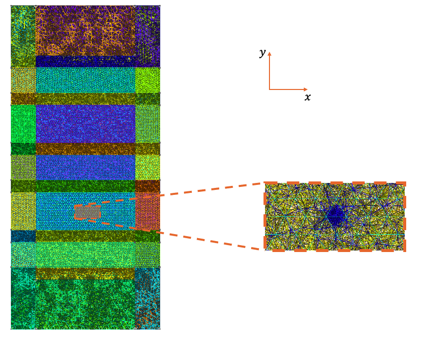
Fig. 20.6.1 Mesh produced by the adaptive meshing algorithm after the addition of a point charge at the interface between the silicon channel and the oxide separating it from the front gates, at the center of plunger gate 1, \((x, y) = (0, -17.5 \, \mathrm{nm})\). Besides the mesh being adapted to more easily solve the non-linear Poisson equation, the mesh is also refined around the point charge to ensure that it is observed by the solvers.
20.7. Schrödinger solver
We also write the function func_schrodinger that applies the Schrödinger
solver to a subdevice of the full FD-SOI device.
This subdevice is defined by the regions that form the double quantum dot.
The function takes a device object as input (i.e. the FD-SOI device generated
by func_poisson) and returns the subdevice object over which the
Schrödinger equation has been solved.
def func_schrodinger(d: Device) -> SubDevice:
    """ Apply the Schrodinger solver to the double-dot region of the FD-SOI
    device.

    Args:
        d (Device): An FD-SOI device over which the non-linear Poisson
            solver has been applied.

    Returns:
        SubDevice: The subdevice object over which the Schödinger equation
            has been solved.
    """

    d.set_V_from_phi()

    # List of regions forming the double quantum dot region
    dot_region_list = [
        "oxide_dot", "gate_oxide_dot", "buried_oxide_dot", "channel_dot"
    ]
    # Create a submesh including only the dot region
    submesh = SubMesh(d.mesh, dot_region_list)
    # Create a subdevice object
    subdevice = SubDevice(d, submesh)

    # Configure the Schrodinger solver
    solver_params               = SchrodingerSolverParams()
    solver_params.num_states    = 10
    solver_params.tol           = 1e-6

    # Solve Schrodinger
    slv = SchrodingerSolver(subdevice, solver_params=solver_params)
    slv.solve()

    return subdevice
20.8. Generate data
Now that we have created the two functions described above, we solve the
Poisson and Schrödinger equations while varying the position of a single point
charge to determine the effect of the point-charge position on the quantum-dot
spectrum.
In this example, we place a single point charge, \(Q = e\), at \(z=0\),
the interface between the undoped silicon channel and the oxide that separates
it from the front gates and vary its in-plane position using a The for statement loop for
each in-plane coordinate.
# Generate data ---------------------------------------------------------------

def generate_data(prof, save_file) -> None:
    """ Compute the eigenergies of the FD-SOI as a function of the position
    of a point charge.

    Args:
        prof (str): Profile of the point charge.
        save_file (str): File to save the data.

    """

    # Loop over point-charge positions
    npts_dir    = 3         # Number of points per direction
    x0, y0      = 0, -17.5  # Center of plunger gate 1
    xmin, ymin  = -20, -25  # Minimum position

    x_var       = np.linspace(xmin, x0, npts_dir)
    x_const     = x0 * np.ones(npts_dir)
    y_var       = np.linspace(ymin, y0, npts_dir)
    y_const     = y0 * np.ones(npts_dir)

    x_values    = np.append(x_var[0:npts_dir-1], x_const)
    y_values    = np.append(y_const[0:npts_dir-1], y_var)

    for i, x in enumerate(x_values):
        y = y_values[i]

        pos = np.array([[x, y, 0]]) * scaling       # position of the point charge
        Q = np.array([1]) * ct.e                    # charge of the point charge
        r = 1e-10                                   # radius of the point charge

        dvc = func_poisson(pos, Q, r, prof=prof)    # Solve Poisson
        subdevice = func_schrodinger(dvc)           # Solve Schrodinger

        subdevice.print_energies()                  # Print energies

        # Save energies
        out = np.append(np.array([x, y]), subdevice.energies / ct.e)
        # header
        E_header = '' # set empty header
        if not os.path.isfile(save_file): # checks if the file exists
            # if it doesn't then add the header
            E_header = "x (nm), y (nm), energies (eV)"
        with open(save_file, 'a') as file:
            np.savetxt(file, np.array(out)[np.newaxis, :], header = E_header)
The function defined above generates the data for different point-charge
density profiles, specified with the profile argument.
It computes the eigenenergies of the FD-SOI device as a function of the
position of a point charge and saves the results in a text file, save_file
for potential future use.
At the end of this loop, the file will contain the results of 5 calculations,
each corresponding to a different point-charge position.
This is expected to take ~10 minutes to run on a modern laptop.
20.9. Visualizing the results
We also create a function that allows us to visualize the results. It takes as inputs the file where the data was saved and the file where the plot will be saved.
# Visualize data --------------------------------------------------------------

def visualize_data(E_file, Delta_file) -> None:
    """ Visualize the data generated by the generate_data function.

    Args:
        E_file (str): File containing the data.
        Delta_file (str): File to save the plot.
    """

    # Load the data
    data = np.loadtxt(E_file)
    x = data[:, 0]
    y = data[:, 1]
    gap = data[:, 3] - data[:, 2]

    # Plot labels
    label = '$\Delta E$ (eV)'
    title = 'Orbital level spacing'
    xlabel = '$x$ (nm)'
    ylabel = '$y$ (nm)'

    # Create figure and axes
    fig, ax = plt.subplots(figsize=(8, 6))

    # Plot the data
    scatter = ax.scatter(x, y, c=gap, cmap='viridis')
    fig.colorbar(scatter, ax=ax, label=label)

    # Set labels
    ax.set_title(title)
    ax.set_xlabel(xlabel)
    ax.set_ylabel(ylabel)
    ax.grid(True)

    # Display the plot
    plt.savefig(str(Delta_file))
    plt.show()
This function creates the gap variable which contains the energy gap
between the ground and first excited states for every point-charge position.
We then plot the energy gap between the ground and first excited states as a
function of the point-charge position.
The colorbar corresponds to the energy gap between the ground and first excited
states and the x and y axes correspond to the in-plane position of the point
charge (see Fig. 20.10.1).
20.10. Calculation
Now that all the functions are setup, we perform the calculation. We start with the Gaussian profile.
if __name__ == '__main__':

    # Generate data
    profile = 'Gaussian'
    generate_data(profile, E_file_G)

    # Visualize data
    visualize_data(E_file_G, Delta_file_G)
The results are shown in Fig. 20.10.1.

Fig. 20.10.1 Orbital level spacing as a function of the point-charge position for the quantum dot located below plunger gate 1. The point-charge density profile is Gaussian. The computational time for this example is ~10 minutes on a modern laptop.
The center of plunger gate 1 is located at \((x, y) = (0, -17.5 \, \mathrm{nm})\). The peak of the ground-state wavefunction and the node of the excited-state wavefunction coincides with this point (see Fig. 20.5.1 and Fig. 20.5.2). Accordingly, the energy gap between the ground and first excited states is largest when a point charge is placed at this position and is a factor of 2 larger than the gap when the point charge is far from the center.
We then perform the same calculation using the profile generated in the MVEMT applied to a donor in silicon tutorial. This profile was computed by solving the multi-valley effective-mass theory Schrödinger equation (see Multivalley effective-mass theory solver) for a phosphorus donor in silicon. We load the profile that was saved in the MVEMT applied to a donor in silicon tutorial and repeat the calculation.
Note
Because the following lines of code require the output from the MVEMT applied to a donor in silicon tutorial, if it has not yet been run, comment out the following lines of code.
donor = load(donor_profile_file)
# Generate data
profile = donor
generate_data(profile, E_file_D)

# Visualize data
visualize_data(E_file_D, Delta_file_D)
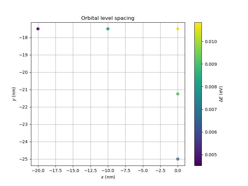
Fig. 20.10.2 Orbital level spacing as a function of the point-charge position for the quantum dot located below plunger gate 1. The point-charge density profile is that of a phosphorus donor in silicon, loaded from the output of the MVEMT applied to a donor in silicon tutorial. The computational time for this example is ~10 minutes on a modern laptop.
Comparing the colorbars of Fig. 20.10.1 and Fig. 20.10.2,
it seems that the maximal energy gap between the ground and first excited
states is larger for the donor profile than for the Gaussian profile.
However, the Gaussian profile has a length scale set by r = 1e-10 (i.e. 1
Angstrom), which is much smaller than the length scale of the donor profile
(which is on the order of nm).
The smaller length scale of the Gaussian profile is associated with larger
charge densities which we expect to lead to larger energy gaps.
However as mentioned in the MVEMT applied to a donor in silicon tutorial, the donor wavefunctions
have not been converged with respect to the size and resolution of the mesh.
This is likely the reason for the discrepancy between our expectation and the
calculated values.
(In particular, because the sphere over which the donor wavefunctions were
calculated is too small, we expect the associated charge density to be larger
than expected).
Note
We have performed a similar calculation using the parameters mentioned
in the MVEMT applied to a donor in silicon that lead to convergence of the donor wavefunctions.
The results with the converged mesh match our expectations.
That is to say, the energy gap between the ground and first excited state
that is smaller than that obtained with the Gaussian profile with
r=1e-10.
Note
A more complete idea of the dependence of the orbital level spacing of the dot situated beneath plunger gate 1 as a function of the point charge position can be obtained by computing the spectrum at more points. For a more complete example (which took substantially more time to compute), see Fig. 20.10.3.
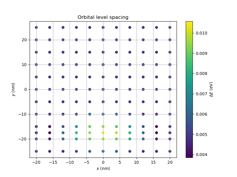
Fig. 20.10.3 Orbital level spacing as a function of the point-charge position for the quantum dot located below plunger gate 1. The point-charge density profile is Gaussian. More data is presented here than in Fig. 20.10.1. This plot took substantially more time to compute.
20.11. Full code
__copyright__ = "Copyright 2022-2026, Nanoacademic Technologies Inc."

import numpy as np
import matplotlib.pyplot as plt
import pathlib
import os
from joblib import load
from qtcad.device.mesh3d import Mesh, SubMesh
from qtcad.device.device import Device, SubDevice
from qtcad.device.poisson import Solver, SolverParams
from qtcad.device.schrodinger import Solver as SchrodingerSolver
from qtcad.device.schrodinger import SolverParams as SchrodingerSolverParams
from qtcad.device import constants as ct
from helper.double_dot_fdsoi import get_double_dot_fdsoi

# Files -----------------------------------------------------------------------
script_dir = pathlib.Path(__file__).parent.resolve()

path_mesh = script_dir / "meshes"
path_out = script_dir / "output"

mesh_file = str(path_mesh / "dqdfdsoi.msh")
geo_file = str(path_mesh / "dqdfdsoi.xao")
ref_file = str(path_mesh / "refined_dqdfdsoi_oxide.msh")
donor_profile_file = str(path_out / "pc_density_profile_0.050_4.0.joblib")

E_file_G = str(path_out / "fdsoi_energies_oxide_charge_G.txt")
Delta_file_G = str(path_out / "DeltaE_oxide_G.png")
E_file_D = str(path_out / "fdsoi_energies_oxide_charge_D.txt")
Delta_file_D = str(path_out / "DeltaE_oxide_D.png")

# Setup -----------------------------------------------------------------------

# Load the mesh
scaling = 1e-9
mesh = Mesh(scaling, mesh_file)

# Define the gate bias parameters
back_gate_bias = -0.5
barrier_gate_1_bias = 0.5
plunger_gate_1_bias = 0.7
barrier_gate_2_bias = 0.5
plunger_gate_2_bias = 0.6
barrier_gate_3_bias = 0.5


# Poisson ---------------------------------------------------------------------
def func_poisson(pos: np.ndarray, Q: np.ndarray, r: float, prof="Gaussian") -> Device:
    """Apply the adaptive non-linear Poisson solver with point charges.
    Args:
        pos (np.ndarray): Position of the point charges
        Q (np.ndarray): Charge of the point charges
        r (float): Smearing radius of the point charges
        prof (str): Profile of the point charges
    Returns:
        device: Device over which the non-linear Poisson solver has been
            applied (point charges have been included).
    """

    # Define the device object from the function defined in the FD-SOI tutorial
    dvc = get_double_dot_fdsoi(
        mesh,
        back_gate_bias,
        barrier_gate_1_bias,
        plunger_gate_1_bias,
        barrier_gate_2_bias,
        plunger_gate_2_bias,
        barrier_gate_3_bias,
    )

    dvc.add_point_charges(pos, Q, r=r, refine=True, profile=prof)

    # Configure the Non-Linear Poisson solver
    solver_params = SolverParams()
    solver_params.tol = 1e-3
    solver_params.initial_ref_factor = 0.1
    solver_params.final_ref_factor = 0.75
    solver_params.min_nodes = 50000
    solver_params.max_nodes = 1e5
    solver_params.maxiter_adapt = 30
    solver_params.maxiter = 200
    solver_params.refined_region = [
        "oxide_dot",
        "gate_oxide_dot",
        "buried_oxide_dot",
        "channel_dot",
    ]
    solver_params.h_refined = 0.8
    solver_params.refined_mesh_filename = ref_file

    # Solve Poisson
    slv = Solver(dvc, solver_params=solver_params, geo_file=geo_file)
    slv.solve()

    return dvc


def func_schrodinger(d: Device) -> SubDevice:
    """Apply the Schrodinger solver to the double-dot region of the FD-SOI
    device.

    Args:
        d (Device): An FD-SOI device over which the non-linear Poisson
            solver has been applied.

    Returns:
        SubDevice: The subdevice object over which the Schödinger equation
            has been solved.
    """

    d.set_V_from_phi()

    # List of regions forming the double quantum dot region
    dot_region_list = ["oxide_dot", "gate_oxide_dot", "buried_oxide_dot", "channel_dot"]
    # Create a submesh including only the dot region
    submesh = SubMesh(d.mesh, dot_region_list)
    # Create a subdevice object
    subdevice = SubDevice(d, submesh)

    # Configure the Schrodinger solver
    solver_params = SchrodingerSolverParams()
    solver_params.num_states = 10
    solver_params.tol = 1e-6

    # Solve Schrodinger
    slv = SchrodingerSolver(subdevice, solver_params=solver_params)
    slv.solve()

    return subdevice


# Generate data ---------------------------------------------------------------


def generate_data(prof, save_file) -> None:
    """Compute the eigenergies of the FD-SOI as a function of the position
    of a point charge.

    Args:
        prof (str): Profile of the point charge.
        save_file (str): File to save the data.

    """

    # Loop over point-charge positions
    npts_dir = 3  # Number of points per direction
    x0, y0 = 0, -17.5  # Center of plunger gate 1
    xmin, ymin = -20, -25  # Minimum position

    x_var = np.linspace(xmin, x0, npts_dir)
    x_const = x0 * np.ones(npts_dir)
    y_var = np.linspace(ymin, y0, npts_dir)
    y_const = y0 * np.ones(npts_dir)

    x_values = np.append(x_var[0 : npts_dir - 1], x_const)
    y_values = np.append(y_const[0 : npts_dir - 1], y_var)

    for i, x in enumerate(x_values):
        y = y_values[i]

        pos = np.array([[x, y, 0]]) * scaling  # position of the point charge
        Q = np.array([1]) * ct.e  # charge of the point charge
        r = 1e-10  # radius of the point charge

        dvc = func_poisson(pos, Q, r, prof=prof)  # Solve Poisson
        subdevice = func_schrodinger(dvc)  # Solve Schrodinger

        subdevice.print_energies()  # Print energies

        # Save energies
        out = np.append(np.array([x, y]), subdevice.energies / ct.e)
        # header
        E_header = ""  # set empty header
        if not os.path.isfile(save_file):  # checks if the file exists
            # if it doesn't then add the header
            E_header = "x (nm), y (nm), energies (eV)"
        with open(save_file, "a") as file:
            np.savetxt(file, np.array(out)[np.newaxis, :], header=E_header)


# Visualize data --------------------------------------------------------------


def visualize_data(E_file, Delta_file) -> None:
    """Visualize the data generated by the generate_data function.

    Args:
        E_file (str): File containing the data.
        Delta_file (str): File to save the plot.
    """

    # Load the data
    data = np.loadtxt(E_file)
    x = data[:, 0]
    y = data[:, 1]
    gap = data[:, 3] - data[:, 2]

    # Plot labels
    label = "$\Delta E$ (eV)"
    title = "Orbital level spacing"
    xlabel = "$x$ (nm)"
    ylabel = "$y$ (nm)"

    # Create figure and axes
    fig, ax = plt.subplots(figsize=(8, 6))

    # Plot the data
    scatter = ax.scatter(x, y, c=gap, cmap="viridis")
    fig.colorbar(scatter, ax=ax, label=label)

    # Set labels
    ax.set_title(title)
    ax.set_xlabel(xlabel)
    ax.set_ylabel(ylabel)
    ax.grid(True)

    # Display the plot
    plt.savefig(str(Delta_file))
    plt.show()


if __name__ == "__main__":
    # Generate data
    profile = "Gaussian"
    generate_data(profile, E_file_G)

    # Visualize data
    visualize_data(E_file_G, Delta_file_G)

    donor = load(donor_profile_file)
    # Generate data
    profile = donor
    generate_data(profile, E_file_D)

    # Visualize data
    visualize_data(E_file_D, Delta_file_D)