4. Adaptive-mesh Poisson solver combined with the Schrödinger solver

4.1. Requirements

4.1.1. Software components

• QTCAD

• Gmsh

4.1.2. Geometry file

• qtcad/examples/tutorials/meshes/nanowire_adaptive.geo

4.1.3. Python script

• qtcad/examples/tutorials/adaptive_schrodinger.py

4.1.4. References

• Getting Started

• Poisson solvers

• Poisson and Schrödinger simulation of a nanowire quantum dot

• Poisson solver with adaptive meshing

4.2. Briefing

In this tutorial, we revisit the nanowire structure studied in Poisson and Schrödinger simulation of a nanowire quantum dot, Poisson solver with adaptive meshing, and Poisson solver with background charges. In Poisson solver with adaptive meshing, we saw that a relatively flat potential well (along the symmetry axis of the nanowire) was formed below the Fermi level by the conduction band edge. Here, we will see that the conduction band edge was flat mostly because of screening effects from a classical electron gas forming inside the channel. Due to the nanometric dimensions of the nanowire studied here, this approach is, in fact, inaccurate. This is because the statistical model used to populate the states of the nanowire was classical, and thus neglected quantum confinement.

To study these confinement effects, we will again solve the non-linear Poisson equation self-consistently, but define a “quantum dot region” in which classical charges are set to zero, and where Schrödinger’s equation will be solved. Away from this dot region, charge carriers are still treated classically, enabling numerically efficient computations. In a later tutorial (Many-body analysis of a nanowire quantum dot), we will learn how Coulomb interactions between electrons inside the quantum dot region may be captured in a fully quantum-mechanical way.

4.3. Geometry file

As before, the initial mesh is generated from a geometry file qtcad/examples/tutorials/meshes/nanowire_adaptive.geo by running Gmsh with

gmsh nanowire_adaptive.geo

As in Poisson solver with adaptive meshing, this will produce both .msh4 and .geo_unrolled files, as required by the adaptive-mesh Poisson solver for geometries produced using the built-in Gmsh geometry kernel.

4.4. Setting up the device and the Poisson solver

4.4.1. Header and input parameters

The header and input parameters are almost the same as in the previous tutorial

from qtcad.device import constants as ct
from qtcad.device.mesh3d import Mesh, SubMesh
from qtcad.device import io
from qtcad.device import analysis
from qtcad.device import materials as mt
from qtcad.device import Device, SubDevice
from qtcad.device.poisson import Solver as PoissonSolver
from qtcad.device.poisson import SolverParams
from qtcad.device.schrodinger import Solver as SchrodingerSolver
import pathlib

However, three additional classes are loaded:

• A SubMesh class which will be used to define a subset of the full mesh that will correspond to the dot region.

• A SubDevice class which will be used to define a subset of the full device that will correspond to the dot region.

• The Schrödinger Solver class.

We next define geometry parameters exactly as in the previous tutorial.

# Define some device parameters
Vgs = 2.0                               # Gate-source bias
Ew = mt.Si.chi + mt.Si.Eg/2             # Metal work function
Ltot = 20e-9   # Device height in m
radius = 2.5e-9       # Device radius in m

Finally, we define paths to the mesh and raw geometry files.

# Paths to mesh file and output files
script_dir = pathlib.Path(__file__).parent.resolve()
path_mesh = script_dir / "meshes" / "nanowire_adaptive.msh4"
path_geo = script_dir / "meshes" / "nanowire_adaptive.geo_unrolled"

4.4.2. Loading the initial mesh and defining the device

We load the mesh and define the device exactly as in the previous tutorial.

# Load the mesh
scaling = 1e-9
mesh = Mesh(scaling, path_mesh)

# Create device from mesh and set temperature to 10 mK
d = Device(mesh, conf_carriers="e")
d.set_temperature(10e-3)

# Create device regions
d.new_region('channel_ox',mt.SiO2)
d.new_region('source_ox',mt.SiO2)
d.new_region('drain_ox',mt.SiO2)
d.new_region('channel', mt.Si)
d.new_region('source', mt.Si, pdoping=5e20*1e6, ndoping=0)
d.new_region('drain', mt.Si, pdoping=5e20*1e6, ndoping=0)

# Create device boundaries
d.new_ohmic_bnd('source_bnd')
d.new_ohmic_bnd('drain_bnd')
d.new_gate_bnd('gate_bnd',Vgs,Ew)

4.4.3. Defining the quantum dot region

The dot region will be defined by a union of region labels, here represented by a list.

# Define the dot region as a list of region labels
dot_region = ["channel", "channel_ox"]

It is important to include both the channel and the oxide surrounding it in the dot region because we will need to include the interface between these regions when solving Schrödinger’s equation. Indeed, this interface defines the potential barriers which confine the electrons inside the channel.

We then define the dot region in which no classical charge is allowed using the set_dot_region of the Device class. This must be done before solving Poisson’s equation—otherwise the Poisson solver may put classical charges inside the quantum dot which will lead to screening effects that would not be there if the quantum dot were to contain just a few confined electrons.

# Set up the dot region in which no classical charge is allowed
d.set_dot_region(dot_region)

4.4.4. Setting up the adaptive-mesh Poisson solver

The next step is to set up the parameters of the adaptive-mesh Poisson solver. Here we proceed exactly as in the previous tutorial, except that we set the minimum number of nodes to 10,000 to ensure that the resolution of the final mesh is satisfactory.

In addition, we define two important solver parameters (see the Poisson SolverParams API reference for a more extensive description of these parameters):

• dot_region: a list of strings labeling a collection of regions in which we want to set a maximal value for the characteristic length.

• h_dot: the maximal value for the characteristic length.

Importantly, setting the dot_region solver parameter does not set classical charge to zero (this was done above with the set_dot_region of the Device class). Instead, the solver parameters introduced here enable to force the adaptive meshing algorithm to keep the mesh fine enough in the dot region for a satisfactory accuracy in the solution of the Schrödinger equation which will be obtained later.

# Configure the non-linear Poisson solver
params_poisson = SolverParams()
params_poisson.tol = 1e-5 # Convergence threshold (tolerance) for the error
params_poisson.initial_ref_factor = 0.1
params_poisson.final_ref_factor = 0.75
params_poisson.min_nodes = 10000
params_poisson.dot_region = dot_region
params_poisson.h_dot = 0.25

Note

The parameter h_dot is expressed in the units of length assumed in the Gmsh geometry file, and not in SI units. Here, since we took scaling=1e-9 when creating the mesh, this will mean that the maximum characteristic length in the dot region is \(0.25\;\mathrm{nm}\).

After defining Poisson solver parameters, we instantiate the Poisson solver object.

# Create an adaptive-mesh non-linear Poisson solver
s = PoissonSolver(d, solver_params=params_poisson, geo_file=path_geo)

4.5. Solving the Poisson and Schrödinger equations

We launch the Poisson simulation with:

# Self-consistent solution
s.solve()

After convergence of the Poisson solver, we plot the band diagram along the symmetry axis of the nanowire.

# Plot band diagram
analysis.plot_bands(d, (0,0,0), (0,0,Ltot))

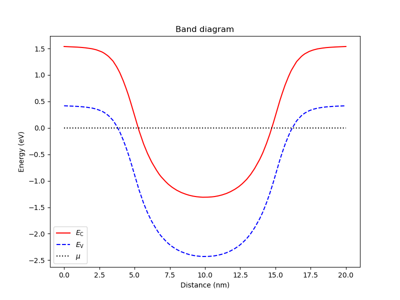
Fig. 4.5.1 Band diagram along the symmetry axis of the nanowire

We note two main differences with the band diagram obtained in Poisson solver with adaptive meshing. (i) The potential well is much deeper. (ii) The bottom of the potential well has a parabolic-like shape. Both differences are related to the fact that screening from a classical gas of electrons in the channel is now absent.

Using the solution of the non-linear Poisson equation, we then define the confinement potential energy which will be used to solve Schrödinger’s equation.

# Get the potential energy from the band edge for usage in the Schrodinger
# solver
d.set_V_from_phi()

The next step is to create a subset of the device in which Schrödinger’s equation will be solved.

We first create a SubMesh object which contains only the nodes inside the dot region.

# Create a submesh including only the dot region
submesh = SubMesh(d.mesh, dot_region)
submesh.show()

The second command above displays the submesh.

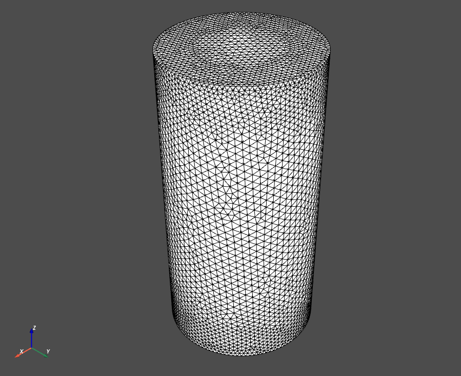
Fig. 4.5.2 Submesh for the dot region

This submesh is non-uniform (finer at the top and bottom boundaries), since it accounts for both the automatic mesh refinements and the maximum characteristic lengths set in the adaptive-mesh Poisson solver parameters.

Once the submesh is created, we define the subset of the device which lives over this submesh.

# Create a subdevice for the dot region
subdevice = SubDevice(d,submesh)

We then instantiate the Schrödinger equation over the subdevice, and solve.

# Create a Schrodinger solver
schrod_solver = SchrodingerSolver(subdevice)

# Solve Schrodinger's equation
schrod_solver.solve()

We print the energy levels obtained from the numerical solution of Schrödinger’s equation (by default, the first ten levels—see the Schrödinger SolverParams API reference to account for a different number of energy levels).

# Print energies
subdevice.print_energies()

The result is

Energy levels (eV)
[-0.89616905 -0.81939494 -0.73555787 -0.64530374 -0.54797826 -0.44382518
-0.33280352 -0.29090282 -0.29038706 -0.21040997]

In this step, We plot the first three eigenfunctions.

# Plot the first three eigenfunctions
analysis.plot_slices(submesh, subdevice.eigenfunctions[:,0],
   title="Ground state")
analysis.plot_slices(submesh, subdevice.eigenfunctions[:,1],
   title="First excited state")
analysis.plot_slices(submesh, subdevice.eigenfunctions[:,2],
   title="Second excited state")

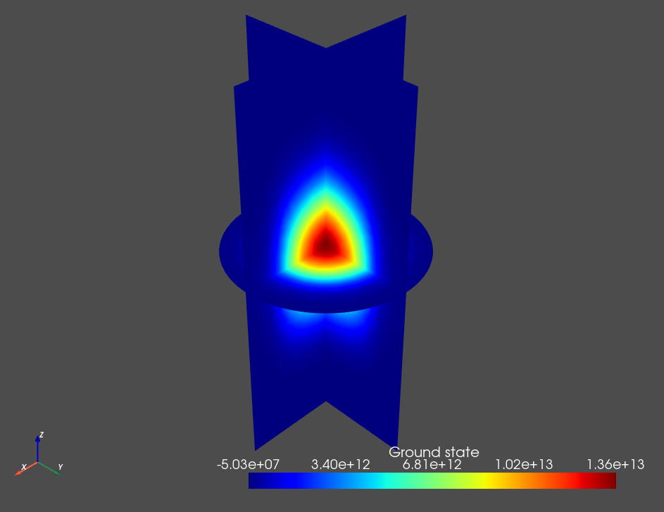
Fig. 4.5.3 Single-electron ground state of the nanowire

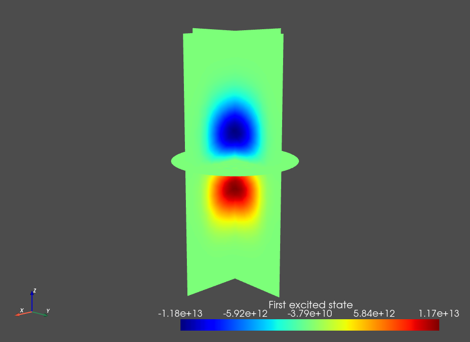
Fig. 4.5.4 Single-electron first excited state of the nanowire

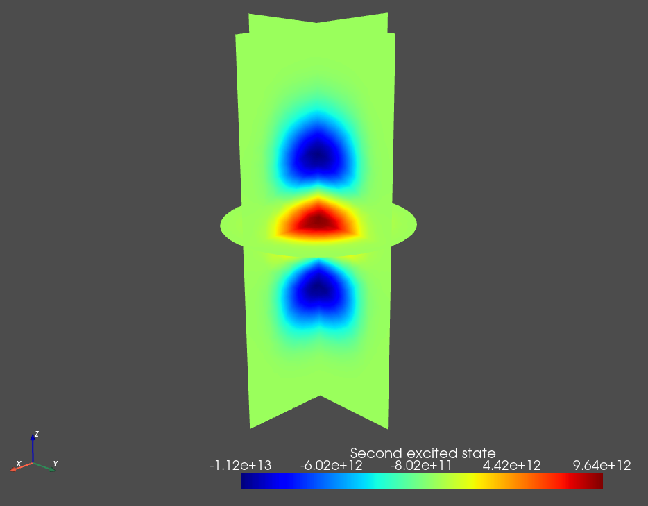
Fig. 4.5.5 Single-electron second excited state of the nanowire

Finally, we produce a 2D plot of a slice of the first eigenfunction in the \(x\)-\(y\) plane for better visualization.

# Define the xy plane for the slice
normal = (0,0,1)
origin = (0,0,1e-8)
# Plot the first eigenfunction in z=10 nm plane.
analysis.plot_slice(submesh, subdevice.eigenfunctions[:,0],
   normal=normal, origin=origin, title="Ground state at $z$=10 nm")

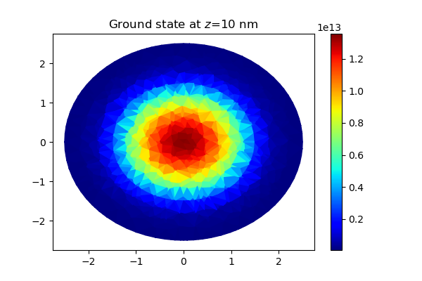
Fig. 4.5.6 A slice of the ground state of the nanowire at \(z = 10\;\mathrm{nm}\)

4.6. Full code

__copyright__ = "Copyright 2022-2024, Nanoacademic Technologies Inc."

from qtcad.device import constants as ct
from qtcad.device.mesh3d import Mesh, SubMesh
from qtcad.device import io
from qtcad.device import analysis
from qtcad.device import materials as mt
from qtcad.device import Device, SubDevice
from qtcad.device.poisson import Solver as PoissonSolver
from qtcad.device.poisson import SolverParams
from qtcad.device.schrodinger import Solver as SchrodingerSolver
import pathlib

# Define some device parameters
Vgs = 2.0                               # Gate-source bias
Ew = mt.Si.chi + mt.Si.Eg/2             # Metal work function
Ltot = 20e-9   # Device height in m
radius = 2.5e-9       # Device radius in m

# Paths to mesh file and output files
script_dir = pathlib.Path(__file__).parent.resolve()
path_mesh = script_dir / "meshes" / "nanowire_adaptive.msh4"
path_geo = script_dir / "meshes" / "nanowire_adaptive.geo_unrolled"

# Load the mesh
scaling = 1e-9
mesh = Mesh(scaling, path_mesh)

# Create device from mesh and set temperature to 10 mK
d = Device(mesh, conf_carriers="e")
d.set_temperature(10e-3)

# Create device regions
d.new_region('channel_ox',mt.SiO2)
d.new_region('source_ox',mt.SiO2)
d.new_region('drain_ox',mt.SiO2)
d.new_region('channel', mt.Si)
d.new_region('source', mt.Si, pdoping=5e20*1e6, ndoping=0)
d.new_region('drain', mt.Si, pdoping=5e20*1e6, ndoping=0)

# Create device boundaries
d.new_ohmic_bnd('source_bnd')
d.new_ohmic_bnd('drain_bnd')
d.new_gate_bnd('gate_bnd',Vgs,Ew)

# Define the dot region as a list of region labels
dot_region = ["channel", "channel_ox"]

# Set up the dot region in which no classical charge is allowed
d.set_dot_region(dot_region)

# Configure the non-linear Poisson solver
params_poisson = SolverParams()
params_poisson.tol = 1e-5 # Convergence threshold (tolerance) for the error
params_poisson.initial_ref_factor = 0.1
params_poisson.final_ref_factor = 0.75
params_poisson.min_nodes = 10000
params_poisson.dot_region = dot_region
params_poisson.h_dot = 0.25

# Create an adaptive-mesh non-linear Poisson solver
s = PoissonSolver(d, solver_params=params_poisson, geo_file=path_geo)

# Self-consistent solution
s.solve()

# Plot band diagram
analysis.plot_bands(d, (0,0,0), (0,0,Ltot))

# Get the potential energy from the band edge for usage in the Schrodinger
# solver
d.set_V_from_phi()

# Create a submesh including only the dot region
submesh = SubMesh(d.mesh, dot_region)
submesh.show()

# Create a subdevice for the dot region
subdevice = SubDevice(d,submesh)

# Create a Schrodinger solver
schrod_solver = SchrodingerSolver(subdevice)

# Solve Schrodinger's equation 
schrod_solver.solve()

# Print energies
subdevice.print_energies()

# Plot the first three eigenfunctions
analysis.plot_slices(submesh, subdevice.eigenfunctions[:,0], 
   title="Ground state")
analysis.plot_slices(submesh, subdevice.eigenfunctions[:,1],
   title="First excited state")
analysis.plot_slices(submesh, subdevice.eigenfunctions[:,2],
   title="Second excited state")

# Define the xy plane for the slice
normal = (0,0,1)
origin = (0,0,1e-8)
# Plot the first eigenfunction in z=10 nm plane.
analysis.plot_slice(submesh, subdevice.eigenfunctions[:,0], 
   normal=normal, origin=origin, title="Ground state at $z$=10 nm")