16. Tunnel coupling in a double quantum dot in FD-SOI—Part 1: Plunger gate tuning

16.1. Requirements

16.1.1. Software components

• QTCAD

• Gmsh

16.1.2. Geometry file

• qtcad/examples/tutorials/meshes/dqdfdsoi.geo

16.1.3. Python script

• qtcad/examples/tutorials/tunnel_coupling_1.py

16.1.4. References

• A double quantum dot device in a fully-depleted silicon-on-insulator transistor

16.2. Briefing

In this tutorial, we will study tunnel coupling in a double quantum dot in the fully-depleted silicon-on-insulator (FD-SOI) geometry introduced in A double quantum dot device in a fully-depleted silicon-on-insulator transistor. We will obtain the detuning between the biases applied on the two plunger gates of the double quantum dot that leads to a symmetric gate bias configuration; the exact meaning of “symmetric” will be clarified in the next section. We will then calculate the tunnel coupling of the double quantum dot.

16.3. Double quantum dot theory

While QTCAD may handle arbitrary confinement potentials numerically, to gain insight into double dot simulation results, it is useful to first study the eigenstates of a single electron in a double quantum dot in a regime in which an analytic model exists.

To gain this theoretical understanding, we focus on the idealized scenario in which the double quantum dot is formed by two potential minima that are well separated, with a large potential barrier between them. In this situation, there exists well-defined single-particle eigenstates for each quantum dot. Identifying the two dots as the “left” and “right” dot, we then label the single-particle ground state of the left and right dots as \(|\mathrm L\rangle\) and \(|\mathrm R\rangle\), respectively.

Neglecting spin, and introducing the detuning \(\Delta E\) between the double dot confinement-potential minima, and introducing the tunnel splitting \(\Omega\), the double quantum dot Hamiltonian may be approximated by [Pla08]:

(16.3.1)\[H = \frac12\left(\Delta E\;\tau_z+\Omega\;\tau_x\right),\]

where we have introduced Pauli matrices in the \(\mathrm L/\mathrm R\) basis:

(16.3.2)\[ \begin{align}\begin{aligned}\tau_x \equiv |\mathrm L\rangle\langle\mathrm R| + |\mathrm R\rangle\langle\mathrm L|,\\\tau_z \equiv |\mathrm L\rangle\langle\mathrm L| - |\mathrm R\rangle\langle\mathrm R|.\end{aligned}\end{align} \]

The Hamiltonian defined by Eq. (16.3.1) can be diagonalized by transforming to the basis of double-dot eigenstates,

(16.3.3)\[ \begin{align}\begin{aligned}|+\rangle &= \cos \frac\theta 2|\mathrm L\rangle + \sin \frac\theta 2|R\rangle,\\|-\rangle &= -\sin \frac\theta 2|\mathrm L\rangle + \cos \frac\theta 2|R\rangle,\end{aligned}\end{align} \]

with associated eigenenergies \(\pm E_d/2\), where

(16.3.4)\[E_d = \sqrt{\Delta E^2 + \Omega^2},\]

and where \(\tan \theta = \Omega /\Delta E\).

The first two double-dot energy levels may then be illustrated as follows.

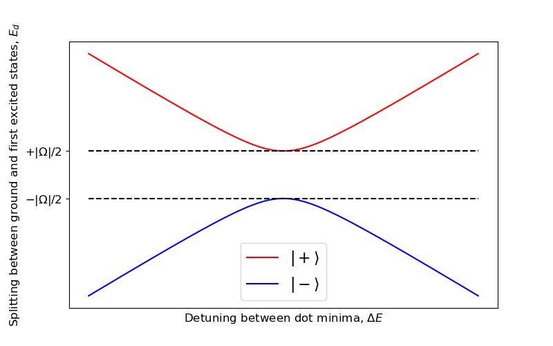
Fig. 16.3.1 Theoretical double quantum dot ground and first excited orbital states.

As may easily be seen from this plot, the tunnel coupling of a double quantum dot may thus be obtained by minimizing the energy difference between its ground and first-excited orbital states.

In practice, this is typically done by tuning the potential difference between the plunger gates of the two dots, since these potentials predominantly control the detuning between the double-dot potential minima.

It is also worth noting that in the symmetric configuration, in which \(\Delta E=0\), the ground and first excited states of the double quantum dot become, for \(\Omega < 0\),

(16.3.5)\[ \begin{align}\begin{aligned}|-\rangle &= (|\mathrm L\rangle + |\mathrm R\rangle)/\sqrt2,\\|+\rangle &= (|\mathrm L\rangle - |\mathrm R\rangle)/\sqrt2,\end{aligned}\end{align} \]

which are often called the bonding and antibonding states, respectively. These states correspond to symmetric and antisymmetric linear combinations of localized ground states of the double quantum dot, respectively.

16.4. Geometry file

As before, the initial mesh is generated from a geometry file qtcad/examples/tutorials/meshes/dqdfdsoi.geo by running Gmsh with

gmsh dqdfdsoi.geo

Akin to Poisson solver with adaptive meshing, this will produce a .msh file. However, in contrast with this previous tutorial, the geometry file that will be produced here will be a .xao file. Indeed, the .xao file format is appropriate for geometries produced using the OpenCASCADE geometry kernel.

16.5. Header

We start by importing the necessary packages, classes, and functions.

import numpy as np
from pathlib import Path
from matplotlib import pyplot as plt
from scipy.optimize import minimize_scalar
from timeit import default_timer as timer
from qtcad.device import constants as ct
from qtcad.device import io
from qtcad.device import analysis as an
from qtcad.device.mesh3d import Mesh, SubMesh
from qtcad.device import SubDevice
from qtcad.device.poisson import Solver as PoissonSolver
from qtcad.device.poisson import SolverParams as PoissonSolverParams
from qtcad.device.schrodinger import Solver as SchrodingerSolver
from qtcad.device.schrodinger import SolverParams as SchrodingerSolverParams
from examples.tutorials.double_dot_fdsoi import get_double_dot_fdsoi

Most of these packages, classes, and functions were seen before. However, we may comment on the following packages and functions:

• timeit: A standard Python package which we will use to time the duration of the simulations.

• minimize_scalar: A Scipy optimization function that we will use to tune the double quantum dot into its symmetic configuration.

• get_double_dot_fdsoi: The function introduced in A double quantum dot device in a fully-depleted silicon-on-insulator transistor to define the double quantum dot Device object

16.6. Setting up the device

We start with setting up paths and loading the mesh.

# Set up paths
script_dir = Path(__file__).parent.resolve()
path_mesh = script_dir / "meshes"
path_geo = path_mesh / "dqdfdsoi.xao"
path_out = script_dir / "output"

# Load the mesh
scaling = 1e-9
file = path_mesh / "dqdfdsoi.msh"
mesh = Mesh(scaling, file)

We then define variables for the biases applied on the gates.

# Define gate biases
back_gate_bias = -0.5
barrier_gate_1_bias = 0.5
plunger_gate_1_bias = 0.59
barrier_gate_2_bias_low = 0.51
barrier_gate_2_bias_high = 0.57
plunger_gate_2_bias = 0.59
barrier_gate_3_bias = 0.5

We note that the gate bias configuration used here has a reflection symmetry (with the second barrier gate as the axis of symmetry).

In addition, we have defined two potential values for the central barrier gate bias: a low bias value used to generate a high potential barrier between the dots, and a high bias value used to generate a low potential barrier between the dots.

We then define a Device object using the get_double_dot_fdsoi function defined in A double quantum dot device in a fully-depleted silicon-on-insulator transistor.

# Define the device
dvc = get_double_dot_fdsoi(mesh, back_gate_bias, barrier_gate_1_bias,
    plunger_gate_1_bias, barrier_gate_2_bias_high, plunger_gate_2_bias,
    barrier_gate_3_bias)

# List of regions forming the double quantum dot region
dot_region_list = ["oxide_dot", "gate_oxide_dot", "buried_oxide_dot",
                    "channel_dot"]

16.7. Basic electrostatics

The next step is to study the basic electrostatics of the device by solving the non-linear Poisson equation in the gate bias configurations defined above, i.e., with both high and low values of the central barrier gate bias.

We do this by defining a SolverParams object for the non-linear Poisson Solver, by constructing this Solver itself, and by running it with the solve method. Here, we use adaptive meshing and set a maximal mesh characteristic length of \(0.8\;\mathrm{nm}\) in the region in which we expect the double quantum dot to form.

# Configure the non-linear Poisson solver
params_poisson = PoissonSolverParams()
params_poisson.tol = 1e-3 # Convergence threshold (tolerance) for the error
params_poisson.initial_ref_factor = 0.1
params_poisson.final_ref_factor = 0.75
params_poisson.min_nodes = 50000
params_poisson.max_nodes = 1e5
params_poisson.maxiter_adapt = 30
params_poisson.maxiter = 200
params_poisson.dot_region = dot_region_list
params_poisson.h_dot = 0.8
params_poisson.refined_mesh_filename = path_mesh / "refined_dqdfdsoi.msh"

# Instantiate Poisson solver
poisson_slv = PoissonSolver(dvc, solver_params=params_poisson,
    geo_file=path_geo)

# Solve in the original gate bias configuration
poisson_slv.solve()

Using these parameters, the mesh is refined once, leading to convergence within roughly ten iterations and less than \(200,000\) nodes.

We then produce a linecut of the conduction band edge along the \(y\) axis (along the channel), \(1\;\mathrm{nm}\) below the interface between the silicon channel and the gate oxide.

# Produce a linecut of the conduction band edge along the channel
x, y, z = dvc.mesh.glob_nodes.T
ymin = np.min(y);   ymax = np.max(y)
distance, linecut_high_bias = an.linecut(dvc.mesh, dvc.cond_band_edge(),
    (0, ymin, -1e-9), (0, ymax, -1e-9))

We then solve the non-linear Poisson equation again in the low central barrier gate bias configuration, and interpolate the conduction band edge again over the same linecut.

# Solve Poisson again at a lower central barrier gate bias
dvc.set_applied_potential("barrier_gate_2_bnd", barrier_gate_2_bias_low)
poisson_slv.solve(initialize=False)

# Produce another linecut of the conduction band edge along the channel
distance, linecut_low_bias = an.linecut(dvc.mesh, dvc.cond_band_edge(),
    (0, ymin, -1e-9), (0, ymax, -1e-9))

When calling the solve method of the non-linear Poisson Solver object, we set the optional argument initialize to False to expedite convergence by using the solution in the previous configuration as an initial guess.

We then plot both low-bias and high-bias linecuts in the same figure.

# Plot the linecuts
fig = plt.figure(figsize=(8,5))
ax = fig.add_subplot(1,1,1)
ax.set_xlabel("Distance along linecut (nm)")
ax.set_ylabel("Conduction band edge, $E_C$ (eV)")
ax.plot(distance/1e-9, linecut_high_bias/ct.e, "-r",
    label=f"Barrier gate 2 bias: {barrier_gate_2_bias_high} V")
ax.plot(distance/1e-9, linecut_low_bias/ct.e, "-b",
    label=f"Barrier gate 2 bias: {barrier_gate_2_bias_low} V")
ax.legend()
plt.show()

This gives:

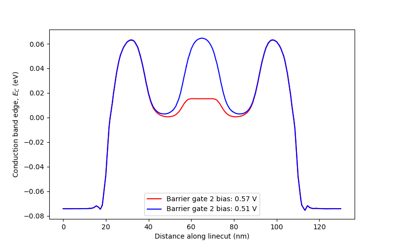
Fig. 16.7.1 Conduction band edge along the channel.

The conduction band edge is well below the Fermi level (the zero of energy, by convention) at the two ends of both linecuts, thus forming source and drain reservoirs containing dense conduction electron gases. Between the source and the drain, we clearly see two potential minima separated from the leads by tall potential barriers, and separated from each other by a central one. While the depth of the potential minima is predominantly controlled by the two plunger gates, the height of the potential barriers is predominantly controlled by the barrier gates. In addition, these potential minima are near the Fermi level, indicating the possibility to load and unload electrons to and from reservoirs, provided that the potential barriers can be sufficiently lowered. The potential barrier between the two minima is high when the central barrier gate bias is low, and low when the central gate bias is high. This will enable to achieve electrostatic control of the tunnel coupling.

While at the scale of Fig. 16.7.1, the conduction band edge appears to be symmetric with respect to the central barrier, a closer inspection reveals numerical noise on the order of \(10\;\mu\mathrm{eV}\) in the vicinity of the potential minima. This can be seen from the plot below, which was achieved by zooming very closely on the minima at high central barrier gate bias in the Pyplot graphical interface.

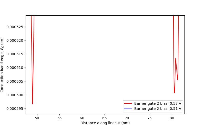
Fig. 16.7.2 Close view of the conduction band edge minima

This numerical noise is asymmetric, and arises from the discretization of the problem over a finite-element mesh. As will be seen later, this can act like an artificial detuning \(\Delta E\) that prevents the ground and first excited state wavefunctions from being the symmetric and antisymmetric states introduced in Eq. (16.3.5), unless an appropriate compensating bias offset is introduced.

Note

While meshes leading to convergence of the non-linear Poisson solver are almost identical between machines and platforms, the exact position and ordering of their nodes can differ slightly. This implies that while the order of magnitude of the numerical asymmetry is expected to be stable, its precise value and behavior may vary between workstations and operating systems. In addition, converging an initial mesh in a slightly different gate bias configuration may lead to slightly different meshes. Therefore, the results obtained in Fig. 16.7.2 may be subject to such variations, and may look slightly different between workstations.

16.8. Tuning the double quantum dot into a symmetric configuration

As explained above, despite the symmetry of the original geometry, numerical asymmetries introduced by the mesh may prevent the formation of symmetric and antisymmetric ground and first excited states, even for perfectly symmetric gate bias configurations. In addition, in an actual experiment, devices are never perfectly symmetric due to the finite precision of fabrication processes and the presence of defects (for example, charges trapped in the oxide regions). Therefore, to evaluate the tunnel coupling of a double quantum dot, it is a good practice, both experimentally and numerically, to tune one of the plunger gates to minimize the splitting between the ground and first excited orbital states. Since artificial detunings due to mesh asymmetries are expected to have the strongest impact at weak tunneling (i.e., when \(\Omega\lesssim \Delta E\)), we minimize the splitting in the low central barrier gate bias configuration (the one in which the Device was just set in the last Poisson simulation), in which the central potential barrier is the highest and thus tunnel coupling the weakest.

To perform this optimization, we first create a SubMesh object that corresponds to the double quantum dot region. It is important to do so after solving the non-linear Poisson equation, since the SubMesh should be defined as a subset of the parent Mesh after its final refinement.

# Create a submesh including only the dot region
submesh = SubMesh(dvc.mesh, dot_region_list)

We continue by instantiating a SolverParams object for a Schrödinger Solver.

# Instantiate Schrodinger solver parameters
params_schrod = SchrodingerSolverParams()
params_schrod.tol = 1e-6 # Tolerance on energies in eV

Here, we will tune the value of the potential applied on plunger gate 2 away from its reference value of \(0.59\;\mathrm{V}\) by a small offset \(x\) to minimize the double dot energy splitting. To do so, we define a function that takes this offset as input and returns the splitting between the ground and first excited orbital states of the double quantum dot as output.

# defining the function for optimization.
def function(x, gate_bias, path_states = None, path_phi = None):
    """ Tunnel splitting to be optimized.

    Args:
        x (float): Gate bias detuning with respect to reference configuration.
        gate_bias (float): Gate bias in the reference configuration.
        path_states (str): Path in which to save the ground and first
            excited state wavefunctions in .vtu format. If None, do not save.
        path_phi (str): Path in which to save the electric potential in .hdf5
            format.

    Returns:
        float: The tunnel splitting (in eV).

    """

    print("="*80)
    print("Evaluating double-dot splitting for detuning: {} V".format(x))
    print("="*80)

    # Set the plunger gate bias
    dvc.set_applied_potential("plunger_gate_2_bnd", gate_bias + x)

    # Solve the non-linear Poisson equation
    poisson_slv.solve(initialize=False)

    # Get the potential energy from the band edge for usage in the Schrodinger
    # solver
    dvc.set_V_from_phi()

    # Create a subdevice for the dot region
    subdvc = SubDevice(dvc, submesh)

    # Instantiate and run a Schrödinger solver
    schrodinger_slv = SchrodingerSolver(subdvc, solver_params = params_schrod)
    schrodinger_slv.solve()

    # Store the solution as an initial guess for the next run
    params_schrod.guess = (subdvc.eigenfunctions, subdvc.energies)

    energies = subdvc.energies

    if path_states is not None:
        out_dict = {
            "Ground state": subdvc.eigenfunctions[:,0],
            "First excited state": subdvc.eigenfunctions[:,1]
        }
        io.save(path_states, out_dict, submesh)

    if path_phi is not None:
        out_dict = {"phi": dvc.phi}
        io.save(path_phi, out_dict)

    return (energies [1] - energies [0])/ct.e

In this function, we first apply the offset potential to plunger gate 2, and solve the non-linear Poisson equation in this updated bias configuration to find the corresponding electric potential. The corresponding confinement potential is then updated from this electric potential by calling set_V_from_phi. The next step is to create a SubDevice object corresponding to the dot region, over which a single-electron Schrödinger solver is then instantiated and solved. The resulting energy splitting between the ground and first excited state is then returned, unless optional paths to output files were given, in which case the electric potential in .hdf5 format and the ground and first excited state wavefunctions in .vtu format may be output first.

Note

Here, when calling the solve method of the Poisson Solver, we set the optional argument initialize to False. This is to avoid resetting the potential across the device into the default initial guess of the non-linear Poisson solver and to use the values currently stored in the phi attribute of the device instead. Likewise, we store the eigenfunctions and eigenenergies that result from the Schrödinger solution into the guess attribute of the Schrödinger SolverParams object for further use in subsequent Schrödinger runs. These two steps greatly speed up convergence of both Poisson and Schrödinger solvers when only slightly changing an applied bias between successive runs.

After defining the function to be minimized, we proceed with the actual minimization procedure. To do so, we use a SciPy function called minimize_scalar. Two optimization methods are suggested to find the optimal plunger gate bias offset:

• The bounded method, which requires specifying a range for the variable \(x\) to be optimized.

• The brent method, which does not require a range.

Using the bounded method can result into fast convergence to the minimum if a sufficiently tight range around the offset value is given. However, this method may be inaccurate if the input range is too broad. In cases in which a range cannot be given for the offset, Brent’s method may be more robust, but may also potentially require more iterations.

To expedite convergence in this tutorial setting, we use the bounded method with a range of \(\pm 200\;\mu\mathrm{V}\). We also set the tolerance on the bias offset to \(10^{-7}\;\mathrm{V}\).

# Tune the bias of plunger gate 2 to find a symmetric double dot
# configuration
t0 = timer()
result = minimize_scalar(function, bounds=(-200e-6,200e-6), args=(
    np.array([plunger_gate_2_bias])), method = 'bounded',
    options={"xatol": 1e-7})

# print results:
print (f'Optimum found at {result.x} V with the value: {result.fun} eV.')
print(f'Computation time: {timer()-t0} s')

# Save the optimum and detuning in a file
path_result = path_out / "detuning_and_coupling.txt"
tab = np.array([result.x, result.fun])
np.savetxt(path_result, tab)

We also count the time required (in seconds) for the optimal offset to be found. This time can be expected to be of the order of five to ten minutes on a typical (modern) laptop. In addition, we save the final plunger gate bias offset and energy splitting into a text file. These quantities are also printed in the standard output. We find:

Optimum found at 6.587085284689152e-06 V with the value: 1.2931073226197486e-06 eV.

This means that the tunnel coupling of our double quantum dot is \(1.29\;\mu\mathrm{eV}\). While this value of the coupling should be similar on different machines, the value of the offset may vary significantly, since the origin of the offset is the asymmetry of the potentials which is not physical, but arises from numerical precision of the mesh and of the solvers.

Finally, once the optimal configuration is found, we call the function two last times with optional arguments for the output file paths to save the electric potential in the high barrier configuration, and the ground and first excited state wavefunctions in the high and low barrier configurations. While the electric potential in the high barrier configuration will be used in the next tutorial to save computation time in an initial non-linear Poisson run, the wavefunctions may be visualized in 3D using ParaView in both configurations.

# Save the ground and first excited state wave functions in .vtu format
# Save the electric potential in .hdf5 format
print("Solving Poisson and Schrödinger for the final detuning value.")
print("Saving eigenfunctions in .vtu format.")
path_states = str(path_out / "tunnel_coupling_wavefunctions_high_barrier.vtu")
path_phi = str(path_out / "tunnel_coupling_final_potential.hdf5")
function(result.x, np.array(plunger_gate_2_bias), path_states=path_states,
    path_phi=path_phi)

# Save the ground and first excited state wave functions in .vtu format
# at high central barrier gate bias (strong tunneling)
dvc.set_applied_potential("barrier_gate_2_bnd", barrier_gate_2_bias_high)
path_states = str(path_out / "tunnel_coupling_wavefunctions_low_barrier.vtu")
function(result.x, np.array(plunger_gate_2_bias), path_states=path_states)

By taking a clipping along the plane perpendicular to the \(x\) axis, we may see that the ground and first excited state wavefunctions correspond to the bonding and antibonding states introduced in Eq. (16.3.5). In addition, we remark that, as expected, the lobes of these bonding and antibonding states have stronger overlap in the low central barrier configuration, corresponding to stronger tunnel coupling.

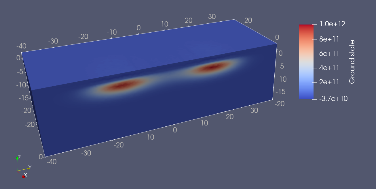
Fig. 16.8.1 Double quantum dot ground state in the high central barrier gate bias (low barrier height) configuration.

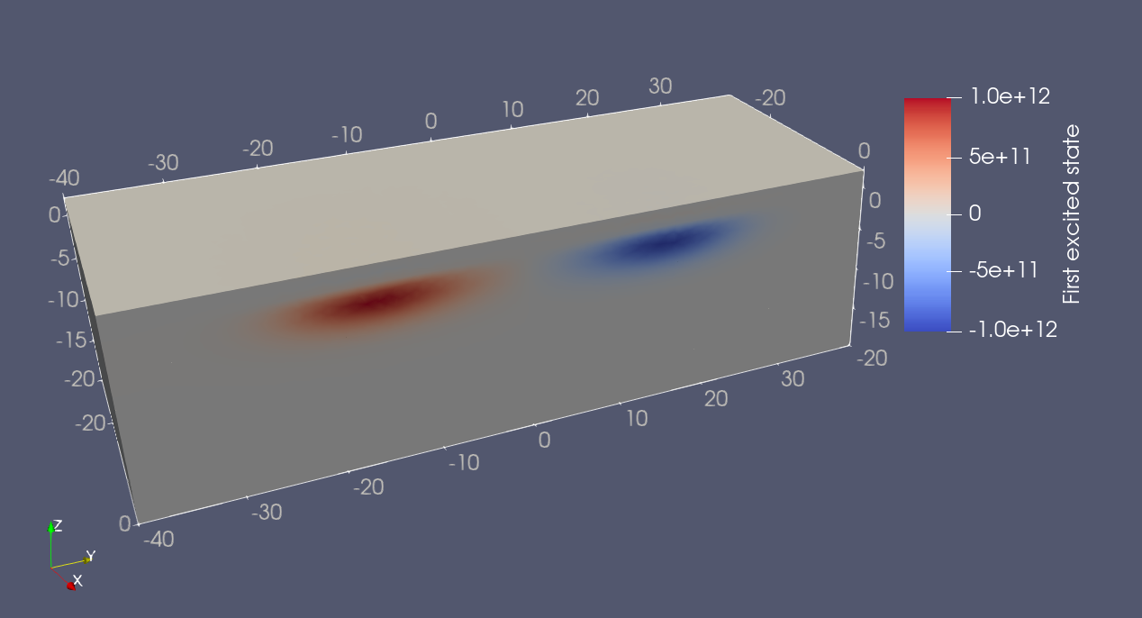
Fig. 16.8.2 Double quantum dot first excited state in the high central barrier gate bias (low barrier height) configuration.

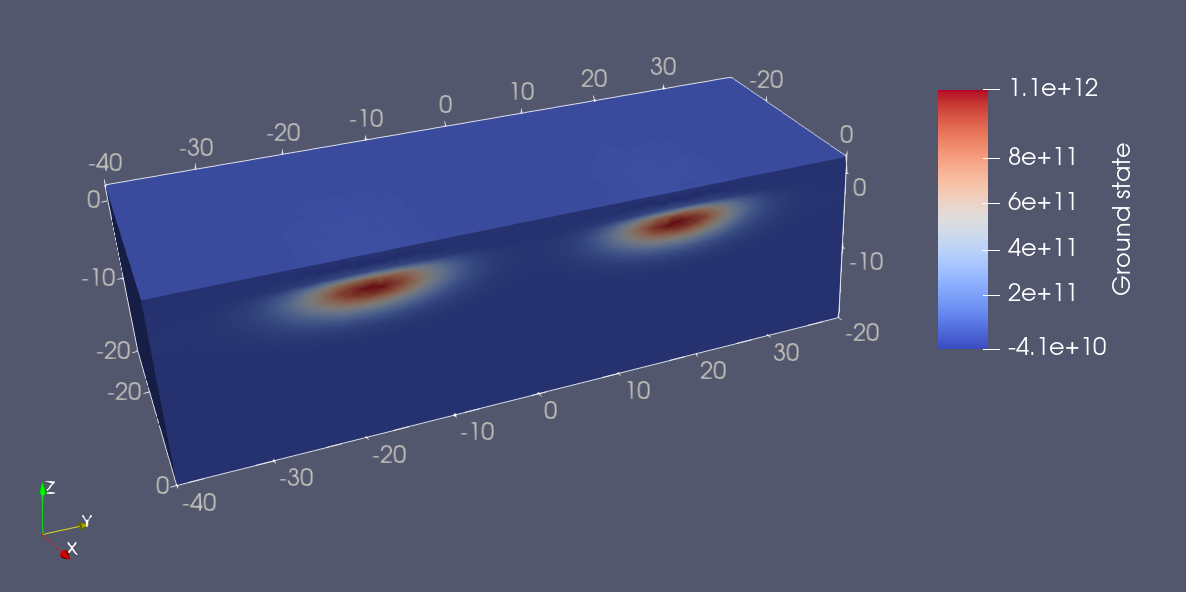
Fig. 16.8.3 Double quantum dot ground state in the high central barrier gate bias (high barrier height) configuration.

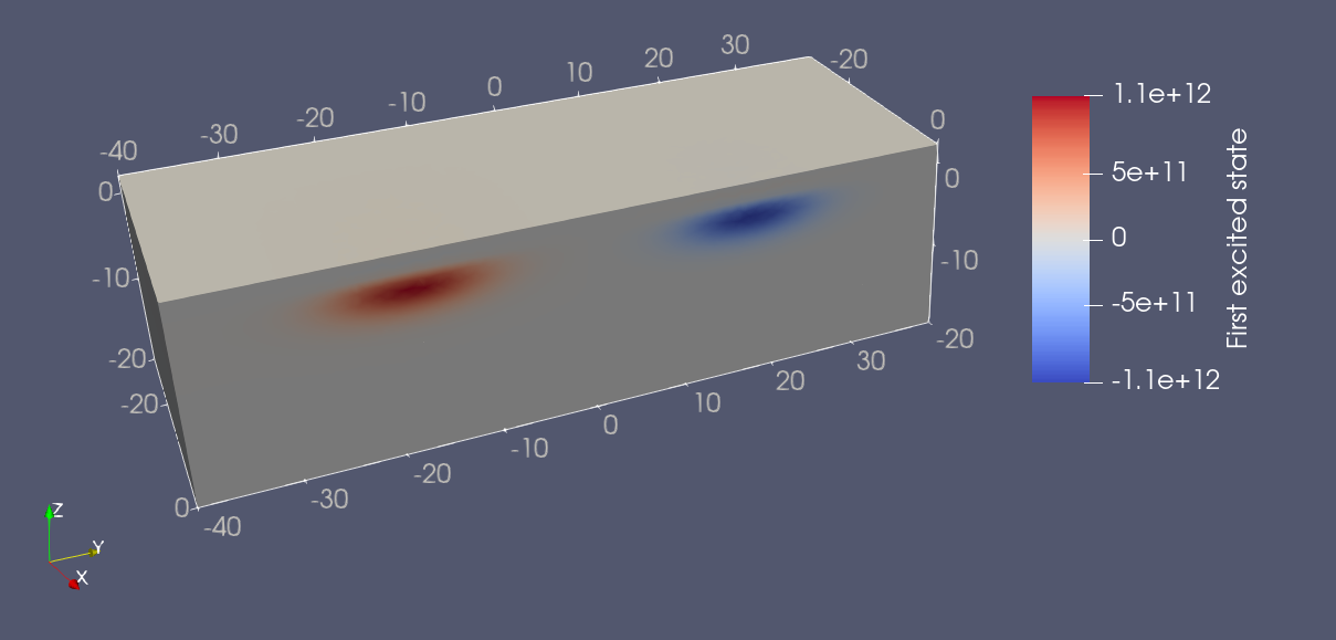
Fig. 16.8.4 Double quantum dot first excited state in the high central barrier gate bias (low barrier height) configuration.

16.9. Full code

__copyright__ = "Copyright 2022-2024, Nanoacademic Technologies Inc."

import numpy as np
from pathlib import Path
from matplotlib import pyplot as plt
from scipy.optimize import minimize_scalar
from timeit import default_timer as timer
from qtcad.device import constants as ct
from qtcad.device import io
from qtcad.device import analysis as an
from qtcad.device.mesh3d import Mesh, SubMesh
from qtcad.device import SubDevice
from qtcad.device.poisson import Solver as PoissonSolver
from qtcad.device.poisson import SolverParams as PoissonSolverParams
from qtcad.device.schrodinger import Solver as SchrodingerSolver
from qtcad.device.schrodinger import SolverParams as SchrodingerSolverParams
from examples.tutorials.double_dot_fdsoi import get_double_dot_fdsoi

# Set up paths
script_dir = Path(__file__).parent.resolve()
path_mesh = script_dir / "meshes"
path_geo = path_mesh / "dqdfdsoi.xao"
path_out = script_dir / "output"

# Load the mesh
scaling = 1e-9
file = path_mesh / "dqdfdsoi.msh"
mesh = Mesh(scaling, file)

# Define gate biases
back_gate_bias = -0.5
barrier_gate_1_bias = 0.5
plunger_gate_1_bias = 0.59
barrier_gate_2_bias_low = 0.51
barrier_gate_2_bias_high = 0.57
plunger_gate_2_bias = 0.59
barrier_gate_3_bias = 0.5

# Define the device
dvc = get_double_dot_fdsoi(mesh, back_gate_bias, barrier_gate_1_bias, 
    plunger_gate_1_bias, barrier_gate_2_bias_high, plunger_gate_2_bias, 
    barrier_gate_3_bias)

# List of regions forming the double quantum dot region
dot_region_list = ["oxide_dot", "gate_oxide_dot", "buried_oxide_dot", 
                    "channel_dot"]

# Configure the non-linear Poisson solver
params_poisson = PoissonSolverParams()
params_poisson.tol = 1e-3 # Convergence threshold (tolerance) for the error
params_poisson.initial_ref_factor = 0.1
params_poisson.final_ref_factor = 0.75
params_poisson.min_nodes = 50000
params_poisson.max_nodes = 1e5
params_poisson.maxiter_adapt = 30
params_poisson.maxiter = 200
params_poisson.dot_region = dot_region_list
params_poisson.h_dot = 0.8
params_poisson.refined_mesh_filename = path_mesh / "refined_dqdfdsoi.msh"

# Instantiate Poisson solver
poisson_slv = PoissonSolver(dvc, solver_params=params_poisson, 
    geo_file=path_geo)

# Solve in the original gate bias configuration
poisson_slv.solve()

# Produce a linecut of the conduction band edge along the channel
x, y, z = dvc.mesh.glob_nodes.T
ymin = np.min(y);   ymax = np.max(y)
distance, linecut_high_bias = an.linecut(dvc.mesh, dvc.cond_band_edge(),
    (0, ymin, -1e-9), (0, ymax, -1e-9))

# Solve Poisson again at a lower central barrier gate bias
dvc.set_applied_potential("barrier_gate_2_bnd", barrier_gate_2_bias_low)
poisson_slv.solve(initialize=False)

# Produce another linecut of the conduction band edge along the channel
distance, linecut_low_bias = an.linecut(dvc.mesh, dvc.cond_band_edge(),
    (0, ymin, -1e-9), (0, ymax, -1e-9))

# Plot the linecuts
fig = plt.figure(figsize=(8,5))
ax = fig.add_subplot(1,1,1)
ax.set_xlabel("Distance along linecut (nm)")
ax.set_ylabel("Conduction band edge, $E_C$ (eV)")
ax.plot(distance/1e-9, linecut_high_bias/ct.e, "-r", 
    label=f"Barrier gate 2 bias: {barrier_gate_2_bias_high} V")
ax.plot(distance/1e-9, linecut_low_bias/ct.e, "-b", 
    label=f"Barrier gate 2 bias: {barrier_gate_2_bias_low} V")
ax.legend()
plt.show()

# Create a submesh including only the dot region
submesh = SubMesh(dvc.mesh, dot_region_list)

# Instantiate Schrodinger solver parameters
params_schrod = SchrodingerSolverParams()
params_schrod.tol = 1e-6 # Tolerance on energies in eV

# defining the function for optimization.
def function(x, gate_bias, path_states = None, path_phi = None):
    """ Tunnel splitting to be optimized.

    Args:
        x (float): Gate bias detuning with respect to reference configuration.
        gate_bias (float): Gate bias in the reference configuration.
        path_states (str): Path in which to save the ground and first 
            excited state wavefunctions in .vtu format. If None, do not save.
        path_phi (str): Path in which to save the electric potential in .hdf5 
            format.

    Returns:
        float: The tunnel splitting (in eV).

    """

    print("="*80)
    print("Evaluating double-dot splitting for detuning: {} V".format(x))
    print("="*80)

    # Set the plunger gate bias
    dvc.set_applied_potential("plunger_gate_2_bnd", gate_bias + x)

    # Solve the non-linear Poisson equation
    poisson_slv.solve(initialize=False)

    # Get the potential energy from the band edge for usage in the Schrodinger
    # solver
    dvc.set_V_from_phi()

    # Create a subdevice for the dot region
    subdvc = SubDevice(dvc, submesh)

    # Instantiate and run a Schrödinger solver
    schrodinger_slv = SchrodingerSolver(subdvc, solver_params = params_schrod)
    schrodinger_slv.solve()

    # Store the solution as an initial guess for the next run
    params_schrod.guess = (subdvc.eigenfunctions, subdvc.energies)

    energies = subdvc.energies

    if path_states is not None:
        out_dict = {
            "Ground state": subdvc.eigenfunctions[:,0],
            "First excited state": subdvc.eigenfunctions[:,1]
        }
        io.save(path_states, out_dict, submesh)

    if path_phi is not None:
        out_dict = {"phi": dvc.phi}
        io.save(path_phi, out_dict)

    return (energies [1] - energies [0])/ct.e

# Tune the bias of plunger gate 2 to find a symmetric double dot
# configuration
t0 = timer()
result = minimize_scalar(function, bounds=(-200e-6,200e-6), args=(
    np.array([plunger_gate_2_bias])), method = 'bounded',
    options={"xatol": 1e-7})

# print results:
print (f'Optimum found at {result.x} V with the value: {result.fun} eV.')
print(f'Computation time: {timer()-t0} s')

# Save the optimum and detuning in a file
path_result = path_out / "detuning_and_coupling.txt"
tab = np.array([result.x, result.fun])
np.savetxt(path_result, tab)

# Save the ground and first excited state wave functions in .vtu format
# Save the electric potential in .hdf5 format
print("Solving Poisson and Schrödinger for the final detuning value.")
print("Saving eigenfunctions in .vtu format.")
path_states = str(path_out / "tunnel_coupling_wavefunctions_high_barrier.vtu")
path_phi = str(path_out / "tunnel_coupling_final_potential.hdf5")
function(result.x, np.array(plunger_gate_2_bias), path_states=path_states,
    path_phi=path_phi)

# Save the ground and first excited state wave functions in .vtu format
# at high central barrier gate bias (strong tunneling)
dvc.set_applied_potential("barrier_gate_2_bnd", barrier_gate_2_bias_high)
path_states = str(path_out / "tunnel_coupling_wavefunctions_low_barrier.vtu")
function(result.x, np.array(plunger_gate_2_bias), path_states=path_states)