9. Schrödinger simulation of a quantum well

9.1. Requirements

9.1.1. Software components

QTCAD
Gmsh

9.1.2. Geometry file

qtcad/examples/tutorials/meshes/qw_1d.geo

9.1.3. Python script

qtcad/examples/tutorials/quantum_well_holes.py

9.1.4. References

9.2. Briefing

In this tutorial, we explain how QTCAD’s Schrödinger solver can be used to simulate structures in lower than three dimensions. An important example is a quantum well where we have confinement along a single direction (\(z\) in our case) and translational invariance along the other two directions (\(x\) and \(y\)). For electrons under the effective mass approximation (where the effective mass is isotropic), this calculation is straightforward. For holes, when there is coupling between bands, it is more complicated and requires projecting the Hamiltonian onto a lower dimension accounting for the wavefunction along the confined dimension. In this tutorial we will calculate the band structure for a hole described by a six-band model [see [For93] for details], bound to a quantum well (1d confinement). We note that the six-band model is only available (for now) for GaAs.

We assume that the user is familiar with basic Python. We also assumed that the user has access to the Gmsh geometry file describing the quantum well. Geometry files for all the QTCAD tutorials are stored in the folder examples/tutorials/meshes.

The full code may be found at the bottom of this page, or in qtcad/examples/tutorials/quantum_well_holes.py.

Do not hesitate to look into the API source code for detailed descriptions of the inputs and outputs of each class, method, or function used in the tutorials. The source code also contains documentation for many other useful features not described here.

9.3. Mesh generation

The mesh is generated from the geometry file qtcad/examples/tutorials/meshes/qw_1d.geo by running Gmsh. This can be done in the terminal with

gmsh qw_1d.geo

This will produce a .msh file in the same directory as the geometry file (quantum_well.msh). See Getting Started for more information about interfacing with Gmsh. Currently, QTCAD only accepts 1D Gmsh meshes along the \(x\) axis.

9.4. Setting up the device

9.4.1. Header

A header is first written to import relevant modules from the QTCAD Device simulator.

from qtcad.device import constants as ct
from qtcad.device import materials as mt
from qtcad.device.mesh1d import Mesh
from qtcad.device import Device
from qtcad.device.schrodinger import Solver, SolverParams


import numpy as np
from matplotlib import pyplot as plt

import pathlib

This block of code imports modules that are necessary to the execution of the remainder of the script. Below is a brief description of what each of these modules is responsible for.

constants: Universal physical constants (elementary charge, Planck’s constant, etc.).
materials: Objects describing each material supported by QTCAD. Here, a material is an object possessing material parameters as attributes. These parameters in include Luttinger parameters, permittivity, effective masses, …
mesh1d: Definition of the 1D Mesh class, which stores information about the position of mesh points, their connectivity (definition of elements, physical regions and boundaries).
device: Definition of the Device class, which is central to all simulations done with QTCAD. A device object stores the value of all physical parameters (effective mass, permittivity, dopant densities, etc.) and variables (electric potential, carrier densities) at each element or mesh point.
schrodinger: Contains the Schrödinger solver which will be used below to find the envelope functions and eigenenergies of holes confined to the quantum well. It can also be used to compute a band structure.

We also import some basic python librairies numpy, matplotlib, and pathlib.

9.4.2. Defining the mesh

The mesh is defined by loading the mesh file produced by Gmsh and setting units of length.

# Paths
path = pathlib.Path(__file__).parent.resolve()
path_mesh = str(path/"meshes"/"quantum_well.msh")

# Load the mesh
scale = 1e-9
mesh = Mesh(scale, path_mesh)

For more details, see e.g. Poisson and Schrödinger simulation of a nanowire quantum dot. Because we have confinement only along 1 direction, we only need a 1d mesh to solve our problem. In the other directions, the system is assumed to be translationally invariant. Thus, the eigenstates are plane waves along these translationally invariant directions and do not need to be solved using QTCAD. We focus here only on the confined part of the states (envelope functions along \(z\)).

9.4.3. Creating the device

The device to simulate is then initialized on the mesh defined above:

# Create the device
# In this example we will consider a 6 valence band model
dvc = Device(mesh, conf_carriers='h',
    hole_kp_model = "luttinger_kohn_foreman_6band")

# Set the material to be GaAs
mat = mt.GaAs
dvc.new_region("well", mat)

# Then create insulator boundaries
dvc.new_insulator("left_barrier")
dvc.new_insulator("right_barrier")

The first line calls the constructor of the device class with the mesh object as an argument. The constructor has two optional arguments. Using the first argument (conf_carriers), we specify that we wish to consider holes confined to the quantum well. Using the second argument (hole_kp_model), we specify the \(\mathbf{k} \cdot \mathbf{p}\) model we will consider for the confined holes. In this case we use the six-band model [For93]. We could also consider the default four-band model by using hole_kp_model = "luttinger_kohn_foreman", or by not specifying the argument at all (in this case, a warning is issued). See k.p module for more details on available models. After the model is specified, we specify the material that hosts our well, GaAs and give boundary conditions. The new_insulator method is used to enforce the boundary conditions of the Schrödinger solver. When solving the Schrödinger eqaution, the solver will look for solutions that vanish at the 'left_barrier' and the 'right_barrier' of the mesh. Since there is no potential defined over the device, we are essentially modelling a particle-in-a-box-like quantum well.

9.5. Solving the Schrödinger solver

9.5.1. Setting up the solver

The parameters of our Schrödinger solver are specified through an instance of a SolverParams object. The num_states attribute indicates we wish to solve for 20 holes states in ascending order, starting from the ground state. We also specify ti_directions which is an attribute that indicates the directions along which we have translational invariance. Here we specify the 'x' and 'y' directions in a list (the device dvc describes the problem along 'z'). We note that while 1D meshes must be defined along the 'x' axis using Gmsh, the ti_directions attribute allows users to specify the confinement (which can be different than 'x') and translationally-invariant directions. In this specific example, the Gmsh mesh defined along the 'x' is reinterpreted by QTCAD to represent a mesh defined along the 'z' axis. Finally, the tol attribute specifies the tolerance of the Schrödinger solver in eV. Here, we reduce it to \(10^{-10}\) compared with the default value \(10^{-6}\), because we observed that a larger tolerance leads to unphysical results in the band structure. More specifically, in the absence of a magnetic field, we expect pairs of spin-degenerate eigenvalues; this property is not respected for the highest energy levels if tolerance is too large.

# Solve Schrodinger's equation
# Parameters
params = SolverParams()
params.num_states = 20
params.ti_directions=['x', 'y']
params.tol = 1e-10
# Solver
s = Solver(dvc, solver_params=params)

9.5.2. Solving the equation

Next, we use the solve method to solve the Schrödinger equation. This method will store the eigenfunctions and eigenenergies in attributes of dvc. As mentioned previously, we are assuming that we have translational invariance along \(x\) and \(y\). Thus, the momentum along each of these two directions (or equivalently, the wavevector) is a good quantum number. Therefore, the Schrödinger equation can, in principle, be solved for any in-plane wavevector \(\mathbf{k} = (k_x, k_y)\). By default, \(\mathbf{k} = (0, 0)\).

# Energies at (0, 0)
s.solve()
print("Energies at (0,0)")
dvc.print_energies()

The print_energies method prints the eigenenergies. The convention used in QTCAD is one where the holes have positive mass and charge (see QTCAD convention for holes for more details).

The solve method can also be used to solve the Schrödinger equation for a different in-plane wavevector. This is done using the keyword argument k.

# Energies at (1, 1)/aB
s.solve(k=np.array([1, 1])/ct.aB, mixing=True)
print("Energies at (1, 1)/aB")
dvc.print_energies()

Here we also solve the Schrödinger equation but for an in-plane wavevector \(\mathbf{k} = a_B^{-1}(1, 1)\), where \(a_B\) is the Bohr radius.

9.5.3. Band Structure

Given that we can solve the Schrödinger equation for different values of \(\mathbf{k}\), we can also compute a band structure for our quantum well.

# Band structure
K = np.linspace(0, 0.3/ct.aB, 30)
basis_vec = np.array([1, 0])

# With mixing
band_structure = s.band_structure(K, basis_vec)

We first specify an array, K, and a basis vector, basis_vec. Together these 2 quantities specify a series of \(\mathbf{k} = k\mathbf{v}\), where \(k\) is an element of K, and \(\mathbf{v}\) represents basis_vec. We pass these two objects into the band_structure method of the solver s. The output is a 2D array that contains the energies of the hole states for every \(\mathbf{k} = k\mathbf{v}\) specified. This output is \(30 \times 20\) in this case: we solve for 20 eigenstates for each of the 30 vectors \(\mathbf{k} = k\mathbf{v}\) specified.

The band_structure can be plotted using basic python plotting functionality

fig = plt.figure(figsize=(7,4))
ax1 = fig.add_subplot(1,1,1)
ax1.plot(K * ct.aB, band_structure/ct.e, '-')
ax1.set_xlabel("$k_x$ ($a_B^{-1}$)")
ax1.set_ylabel("Energy (eV)")
ax1.set_ylim([0, 5])
ax1.set_title("Band structure including band mixing")
plt.show()

Resulting in the following plot:

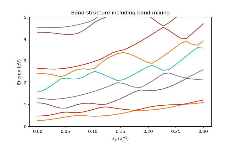
We see from this plot that the bands have positive curvature, consistent with the QTCAD convention for holes.

We can also compute the band structure in the absence of band mixing, i.e. by ignoring all coupling (off diagonal elements) between the valence bands of the model.

# Without mixing
# Compute band structure using QTCAD
band_structure = s.band_structure(K, basis_vec, mixing=False)

This is achieved using the mixing keyword argument of the band_structure method and setting it to False. Before plotting this band structure, we also compute it analytically. This is a straightforward calculation since we are computing particle in a box eigenstates for the confinement along \(z\) and free particle states along \(x\) and \(y\). Since the potential is separable, we can write the total energy as the sum of the energies which solve each of the 1d problems (along \(x\), \(y\), and \(z\) separately).

# Analytic solutions
# Particle in a box energies
def particle_in_box_E(m, L, n):
    return n**2*np.pi**2*ct.hbar**2 / ( 2 * m * L**2 )

g1, g2, g3, Delta = tuple(mat.hole_kp_params)
# Out of plane effective masses
mHH = ct.me / (g1-2*g2) # HH effective mass GaAs
mLH = ct.me / (g1+2*g2) # LH effective mass
mSO = ct.me / g1 # SO effective mass
# In plane effective masses
mHHip = ct.me / (g1 + g2) # HH in-plane effective mass GaAs
mLHip = ct.me / (g1 - g2) # LH in-plane effective mass GaAs
mSOip = ct.me / (g1) # SO in-plane effective mass GaAs

# Analytic energies
PIB_HH = np.array([particle_in_box_E(mHH, 2e-9, n) for n in range(1,5)])
free_HH = ct.hbar**2 / 2 / mHHip * K**2
E_HH = (PIB_HH[np.newaxis, :] + free_HH[:, np.newaxis])

PIB_LH = np.array([particle_in_box_E(mLH, 2e-9, n) for n in range(1,5)])
free_LH = ct.hbar**2 / 2 / mLHip * K**2
E_LH = (PIB_LH[np.newaxis, :] + free_LH[:, np.newaxis])

PIB_SO = np.array([particle_in_box_E(mSO, 2e-9, n) for n in range(1,5)])
free_SO = ct.hbar**2 / 2 / mSOip * K**2
E_SO = (PIB_SO[np.newaxis, :] + free_SO[:, np.newaxis]) + Delta

Here we have defined a function that computes the particle-in-a-box eigenstates. We then get the Luttinger parameters from the material file (in this case mat=mt.GaAs). After computing the in-plane and out-of-plane effective masses for each band, we sum the particle-in-a-box energies and the free electron energies for each band. (We also include the spin-orbit splitting for the split-off band).

Finally, we plot our results.

# Plot
fig = plt.figure(figsize=(7,4))
ax1 = fig.add_subplot(1,1,1)
ax1.plot(K * ct.aB, band_structure/ct.e, '-')
ax1.plot(K * ct.aB, E_HH/ct.e, '--b') # Plot analytic HH energies in blue
ax1.plot(K * ct.aB, E_LH/ct.e, '--r') # Plot analytic LH energies in blue
ax1.plot(K * ct.aB, E_SO/ct.e, '--g') # Plot analytic SO energies in blue
ax1.set_xlabel("$k_x$ ($a_B^{-1}$)")
ax1.set_ylabel("Energy (eV)")
ax1.set_ylim([0, 5])
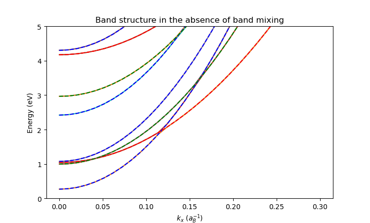
ax1.set_title("Band structure in the absence of band mixing")
plt.show()

We find that the QTCAD solution (solid lines) matches the analytic solution (dashed lines):

9.6. Full code

__copyright__ = "Copyright 2022-2024, Nanoacademic Technologies Inc."

from qtcad.device import constants as ct
from qtcad.device import materials as mt
from qtcad.device.mesh1d import Mesh
from qtcad.device import Device
from qtcad.device.schrodinger import Solver, SolverParams
import numpy as np
from matplotlib import pyplot as plt
import pathlib

# Paths
path = pathlib.Path(__file__).parent.resolve()
path_mesh = str(path/"meshes"/"quantum_well.msh")

# Load the mesh
scale = 1e-9
mesh = Mesh(scale, path_mesh)

# Create the device
# In this example we will consider a 6 valence band model
dvc = Device(mesh, conf_carriers='h',
    hole_kp_model = "luttinger_kohn_foreman_6band")

# Set the material to be GaAs
mat = mt.GaAs
dvc.new_region("well", mat)

# Then create insulator boundaries
dvc.new_insulator("left_barrier")
dvc.new_insulator("right_barrier")

# Solve Schrodinger's equation
# Parameters
params = SolverParams()
params.num_states = 20
params.ti_directions=['x', 'y']
params.tol = 1e-10
# Solver
s = Solver(dvc, solver_params=params)

# Energies at (0, 0)
s.solve()
print("Energies at (0,0)")
dvc.print_energies()


# Energies at (1, 1)/aB
s.solve(k=np.array([1, 1])/ct.aB, mixing=True)
print("Energies at (1, 1)/aB")
dvc.print_energies()

# Band structure
K = np.linspace(0, 0.3/ct.aB, 30)
basis_vec = np.array([1, 0])

# With mixing
band_structure = s.band_structure(K, basis_vec)

fig = plt.figure(figsize=(7,4))
ax1 = fig.add_subplot(1,1,1)
ax1.plot(K * ct.aB, band_structure/ct.e, '-')
ax1.set_xlabel("$k_x$ ($a_B^{-1}$)")
ax1.set_ylabel("Energy (eV)")
ax1.set_ylim([0, 5])
ax1.set_title("Band structure including band mixing")
plt.show()

# Without mixing
# Compute band structure using QTCAD
band_structure = s.band_structure(K, basis_vec, mixing=False)

# Analytic solutions
# Particle in a box energies
def particle_in_box_E(m, L, n):
    return n**2*np.pi**2*ct.hbar**2 / ( 2 * m * L**2 )

g1, g2, g3, Delta = tuple(mat.hole_kp_params)
# Out of plane effective masses
mHH = ct.me / (g1-2*g2) # HH effective mass GaAs
mLH = ct.me / (g1+2*g2) # LH effective mass
mSO = ct.me / g1 # SO effective mass
# In plane effective masses
mHHip = ct.me / (g1 + g2) # HH in-plane effective mass GaAs
mLHip = ct.me / (g1 - g2) # LH in-plane effective mass GaAs
mSOip = ct.me / (g1) # SO in-plane effective mass GaAs

# Analytic energies
PIB_HH = np.array([particle_in_box_E(mHH, 2e-9, n) for n in range(1,5)])
free_HH = ct.hbar**2 / 2 / mHHip * K**2
E_HH = (PIB_HH[np.newaxis, :] + free_HH[:, np.newaxis]) 

PIB_LH = np.array([particle_in_box_E(mLH, 2e-9, n) for n in range(1,5)])
free_LH = ct.hbar**2 / 2 / mLHip * K**2
E_LH = (PIB_LH[np.newaxis, :] + free_LH[:, np.newaxis]) 

PIB_SO = np.array([particle_in_box_E(mSO, 2e-9, n) for n in range(1,5)])
free_SO = ct.hbar**2 / 2 / mSOip * K**2
E_SO = (PIB_SO[np.newaxis, :] + free_SO[:, np.newaxis]) + Delta

# Plot
fig = plt.figure(figsize=(7,4))
ax1 = fig.add_subplot(1,1,1)
ax1.plot(K * ct.aB, band_structure/ct.e, '-')
ax1.plot(K * ct.aB, E_HH/ct.e, '--b') # Plot analytic HH energies in blue
ax1.plot(K * ct.aB, E_LH/ct.e, '--r') # Plot analytic LH energies in blue
ax1.plot(K * ct.aB, E_SO/ct.e, '--g') # Plot analytic SO energies in blue
ax1.set_xlabel("$k_x$ ($a_B^{-1}$)")
ax1.set_ylabel("Energy (eV)")
ax1.set_ylim([0, 5])
ax1.set_title("Band structure in the absence of band mixing")
plt.show()