2. Poisson solver with adaptive meshing
2.1. Requirements
2.1.1. Software components
QTCAD
Gmsh
2.1.2. Geometry file
qtcad/examples/tutorials/meshes/nanowire_adaptive.geo
2.1.3. Python script
qtcad/examples/tutorials/adaptive.py
2.1.4. References
2.2. Briefing
In this tutorial, we explain how to solve Poisson’s equation using an adaptive meshing technique. Adaptive meshing is especially useful at low temperatures (near or below 1K), at which it is often difficult to solve the non-linear Poisson equation with a static mesh.
2.3. Geometry file
As before, a mesh is first generated from a
geometry file qtcad/examples/tutorials/meshes/nanowire_adaptive.geo by
running Gmsh with
gmsh nanowire_adaptive.geo
The nanowire_adaptive.geo file describes exactly the same geometry as the
nanowire.geo file considered in the previous tutorial, but differs in two
important ways:
The
nanowire_adaptive.geofile produces a much coarser mesh, with a uniform characteristic length of 1 nm.While the
nanowire.geofile only produces a single (.msh4) output file, thenanowire_adaptive.geofile also produces a raw Gmsh geometry file with the extension.geo_unrolled. This file will be used as an input to the adaptive Poisson solver.
To produce a .geo_unrolled, it suffices to add the following line of code
at the end of the Gmsh script:
Save "nanowire_adaptive.geo_unrolled";
It is also possible to produce a .geo_unrolled file within the Gmsh GUI
using File > Export; the .geo_unrolled format should be available in the
drop-down menu below the file name.
Note
The .geo_unrolled format is the appropriate raw geometry format to use
here because the nanowire geometry is produced using the built-in Gmsh
geometry kernel. If the geometry is produced using the OpenCASCADE kernel,
the .geo_unrolled format will not be appropriate. In this case, the
geometry should be exported in the .xao format.
2.4. Setting up the device and the Poisson solver
2.4.1. Header and input parameters
The header and input parameters are the same as in the previous tutorial
from qtcad.device import constants as ct
from qtcad.device.mesh3d import Mesh
from qtcad.device import io
from qtcad.device import analysis
from qtcad.device import materials as mt
from qtcad.device import Device
from qtcad.device.poisson import Solver, SolverParams

import pathlib

# Define some device parameters
Vgs = 2.0                               # Gate-source bias
Ew = mt.Si.chi + mt.Si.Eg/2             # Metal work function
Ltot = 20e-9   # Device height in m
radius = 2.5e-9       # Device radius in m
However, in addition to the path to the .msh4 file, we must add a
path to the .geo_unrolled file.
# Paths to mesh file and output files
script_dir = pathlib.Path(__file__).parent.resolve()
path_mesh = script_dir / "meshes" / "nanowire_adaptive.msh4"
path_geo = script_dir / "meshes" / "nanowire_adaptive.geo_unrolled"
2.4.2. Loading the initial mesh and defining the device
The device is first created over the initial (coarse) mesh. Here, we set the temperature to 10 mK.
# Load the mesh
scaling = 1e-9
mesh = Mesh(scaling, path_mesh)

# Create device from mesh and set temperature to 10 mK
d = Device(mesh, conf_carriers="e")
d.set_temperature(10e-3)
We then set up the device regions and boundaries exactly like in Poisson and Schrödinger simulation of a nanowire quantum dot.
# Create device regions
d.new_region('channel_ox',mt.SiO2)
d.new_region('source_ox',mt.SiO2)
d.new_region('drain_ox',mt.SiO2)
d.new_region('channel', mt.Si)
d.new_region('source', mt.Si, pdoping=5e20*1e6, ndoping=0)
d.new_region('drain', mt.Si, pdoping=5e20*1e6, ndoping=0)

# Create device boundaries
d.new_ohmic_bnd('source_bnd')
d.new_ohmic_bnd('drain_bnd')
d.new_gate_bnd('gate_bnd',Vgs,Ew)
2.4.3. Setting up the adaptive-mesh Poisson solver
The next step is to set up the parameters of the Poisson solver.
As in the previous tutorial, this is done through a
SolverParams object.
Here, however, we also specify additional solver parameters that control
adaptive meshing.
# Configure the non-linear Poisson solver
params_poisson = SolverParams()
params_poisson.tol = 1e-5 # Convergence threshold (tolerance) for the error
params_poisson.initial_ref_factor = 0.1
params_poisson.final_ref_factor = 0.75
params_poisson.min_nodes = 0
params_poisson.refined_mesh_filename =\
    script_dir / "meshes" / "nanowire_adaptive_refined.msh4"
As usual, the tolerance attribute
tol
specifies the maximum acceptable potential difference (in volts) between two
successive self-consistent-loop iterations; when this potential difference
is below the tolerance, the self-consistent loop stops and is considered to
have converged. The next three solver parameters control adaptive meshing.
To understand them, we give a brief description of how the adaptive Poisson solver works.
Typically, the initial mesh used for the device is very coarse. For coarse meshes, there is a strong chance that the non-linear Poisson solver does not converge, i.e., that the error on the potential (maximum difference between the potentials in the current and previous iterations) never decreases below tolerance. In this situation we need to refine the mesh. If the Poisson equation still does not converge, the mesh is refined again, repeatedly, until convergence. Remark that automatic refinements account for the electric potential distribution throughout the device, and produce finer meshes in regions of fast variations of the potential to enhance accuracy and convergence.
The SolverParams class API reference
gives a brief description of the adaptive-mesh solver parameters. In particular,
the parameters
initial_ref_factor
and
final_ref_factor
are unitless parameters between \(0\) and \(1\) that control the rate
at which the mesh is refined. A refinement factor close to \(0\) indicates
that the mesh is strongly refined each time convergence fails, while
a refinement factor close to \(1\) indicates that only small refinements
are implemented in these situations. We recommend using a small initial
refinement factor (\(\sim 0.1\)) followed by a large final refinement
factor (\(\sim 0.75\)) (see the default values in the
SolverParams
API reference). With this approach, the mesh size quickly increases in the
beginning, and is then slowly refined to smoothly approach convergence.
Excessively small refinement factors may lead to convergence with less
iterations, but typically also leads to excessive mesh sizes that slow
down computations and waste memory.
Note
A good strategy is often to start with a very coarse initial mesh in which convergence at low temperature is virtually impossible, and then to let the adaptive solver find the mesh that leads to convergence. Starting with an initially fine mesh may lead directly to convergence, but user-defined static meshes are rarely the most accurate because many nodes may be wasted in regions where the electric potential varies smoothly. By contrast, we tend to underestimate the number of nodes required in more difficult regions; it is also very difficult and time consuming to refine the mesh by hand in such problematic regions. Finally, a given mesh may lead to convergence for a certain temperature and gate bias configuration, but slightly changing one of these parameters may cause convergence to fail, in which case automatic mesh adaptation is an advantageous solution.
In addition to the refinement factors, two important adaptive solver parameter
are
min_nodes
and
max_nodes, which
indicate minimum and maximum mesh sizes.
Typically, setting up a maximum number
of nodes is useful in situations in which convergence is difficult and
fast refinements are used, to avoid situations where huge
meshes are generated that cannot be handled by available memory and
computation resources. If no convergence is achieved despite the number of
nodes being above maximum, the simulation stops and an error message is shown.
In this situation, we recommend to try larger values of
initial_ref_factor
and/or
final_ref_factor
to adapt the mesh more slowly but more carefully, and ease convergence.
In situations in which convergence is achieved easily, but in which the mesh is
still too coarse for the results to be considered accurate, it is useful to
set a minimum number of nodes through the
min_nodes
solver parameter. In this case, the mesh refinements will not be allowed to
stop (even if convergence is achieved) until this minimum
number of nodes is used.
It is also possible to set a maximum number of Poisson iterations before the
mesh is adapted through the
maxiter_adapt
parameter, and to define a region with a maximum mesh
characteristic length through the
refined_region
and
h_refined
parameters. This ensures that the mesh is not too coarse in a region of
interest in which, e.g., Schrodinger’s equation will later be solved.
Note
Setting a dot region in the adaptive-mesh solver does not suppress the
charge inside the region. If desired, this feature must be activated
separately by setting a dot region in the
Device object with the
set_dot_region
method.
Finally, the refined_mesh_filename solver parameter specifies the path of
the output mesh file that will be generated at each mesh refinement.
Once the adaptive solver paramerers are configured, the Poisson solver is instantiated with
# Create an adaptive-mesh non-linear Poisson solver
s = Solver(d, solver_params=params_poisson, geo_file=path_geo)
Remark that, in addition to the mandatory
Device argument
and the optional
solver_params argument,
an additional optional argument is provided: the path to the
.geo_unrolled file for the current geometry. This file will provide
information about the device geometry that is necessary for the adaptive solver
to work. If no .geo_unrolled file is specified, a static mesh will be
used (the mesh which is loaded initially).
2.5. Solving Poisson’s equation and analyzing the results
As in Poisson and Schrödinger simulation of a nanowire quantum dot, we launch the calculation with
# Self-consistent solution
s.solve()
The non-linear Poisson solver then iterates using the initial coarse mesh until the error on the electric potential saturates
---
Poisson iteration 10
Maximum absolute error: 0.010741878883199774
Maximum error at (0.000e+00, 0.000e+00, 7.863e-09)
---
Poisson iteration 11
Maximum absolute error: 0.010751709391657926
Maximum error at (0.000e+00, 0.000e+00, 7.863e-09)
---
Poisson iteration 12
Maximum absolute error: 0.010752246271494514
Maximum error at (0.000e+00, 0.000e+00, 7.863e-09)

The error has saturated in the Poisson solver.
Mesh will be refined.
The mesh is then refined, and the Poisson solver runs again until, this time, it converges.
Here, a single mesh refinement is needed because the device geometry is fairly simple. In more complicated geometries, however, a few more rounds of refinement may be needed.
After convergence is achieved, we plot the band diagram along the symmetry axis of the nanowire device.
This is done with
# Plot band diagram
analysis.plot_bands(d, (0,0,0), (0,0,Ltot))
and results in the following figure.
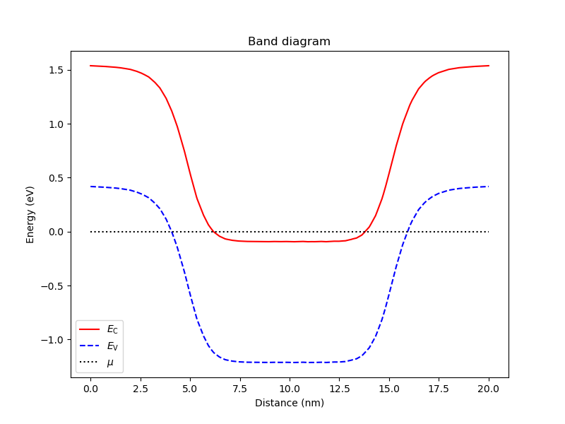
Fig. 2.5.2 Band diagram along the symmetry axis of a nanowire quantum dot using adaptive meshing
If we compare with Fig. 1.5.3, we note that the resulting linecuts look significantly smoother, even though the total number of nodes is almost the same (\(\sim 20,000\) in both cases). This is because the adaptive mesh automatically refines the mesh in regions of fast potential variations but keeps it coarse where the potential varies linearly, and is thus typically much more accurate than manually-genereated meshes for fixed node number.
This can easily be seen by loading the mesh into the Gmsh GUI with
gmsh examples/tutorials/meshes/nanowire_adaptive_refined.msh4
Performing a clipping, coloring by physical groups, and displaying 3D elements, we obtain the following figure, in which we clearly see that the mesh is finer near interfaces between materials or between the channel and the leads, where the potential varies the most non-trivially.
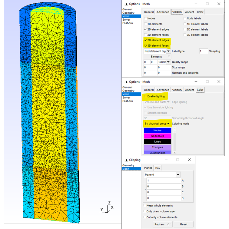
Fig. 2.5.3 Automatically refined mesh (nanowire)
2.6. Full code
__copyright__ = "Copyright 2022-2026, Nanoacademic Technologies Inc."

from qtcad.device import constants as ct
from qtcad.device.mesh3d import Mesh
from qtcad.device import io
from qtcad.device import analysis
from qtcad.device import materials as mt
from qtcad.device import Device
from qtcad.device.poisson import Solver, SolverParams
import pathlib

# Define some device parameters
Vgs = 2.0  # Gate-source bias
Ew = mt.Si.chi + mt.Si.Eg / 2  # Metal work function
Ltot = 20e-9  # Device height in m
radius = 2.5e-9  # Device radius in m

# Paths to mesh file and output files
script_dir = pathlib.Path(__file__).parent.resolve()
path_mesh = script_dir / "meshes" / "nanowire_adaptive.msh4"
path_geo = script_dir / "meshes" / "nanowire_adaptive.geo_unrolled"

# Load the mesh
scaling = 1e-9
mesh = Mesh(scaling, path_mesh)

# Create device from mesh and set temperature to 10 mK
d = Device(mesh, conf_carriers="e")
d.set_temperature(10e-3)

# Create device regions
d.new_region("channel_ox", mt.SiO2)
d.new_region("source_ox", mt.SiO2)
d.new_region("drain_ox", mt.SiO2)
d.new_region("channel", mt.Si)
d.new_region("source", mt.Si, pdoping=5e20 * 1e6, ndoping=0)
d.new_region("drain", mt.Si, pdoping=5e20 * 1e6, ndoping=0)

# Create device boundaries
d.new_ohmic_bnd("source_bnd")
d.new_ohmic_bnd("drain_bnd")
d.new_gate_bnd("gate_bnd", Vgs, Ew)

# Configure the non-linear Poisson solver
params_poisson = SolverParams()
params_poisson.tol = 1e-5  # Convergence threshold (tolerance) for the error
params_poisson.initial_ref_factor = 0.1
params_poisson.final_ref_factor = 0.75
params_poisson.min_nodes = 0
params_poisson.refined_mesh_filename = (
    script_dir / "meshes" / "nanowire_adaptive_refined.msh4"
)

# Create an adaptive-mesh non-linear Poisson solver
s = Solver(d, solver_params=params_poisson, geo_file=path_geo)

# Self-consistent solution
s.solve()

# Plot band diagram
analysis.plot_bands(d, (0, 0, 0), (0, 0, Ltot))