17. Tunnel coupling in a double quantum dot in FD-SOI—Part 2: Tuning the barrier gate
17.1. Requirements
17.1.1. Software components
QTCAD
Gmsh
17.1.2. Geometry file
qtcad/examples/tutorials/meshes/dqdfdsoi.geo
17.1.3. Python script
qtcad/examples/tutorials/tunnel_coupling_2.py
17.1.4. References
17.2. Briefing
This tutorial directly follows Tunnel coupling in a double quantum dot in FD-SOI—Part 1: Plunger gate tuning. In the previous tutorial, we studied a double quantum dot in a generic FD-SOI structure and found two gate bias configurations leading to symmetric and antisymmetric double quantum dot ground and first excited orbital states. These bias configurations corresponded to high central barrier gate bias (leading to a low barrier height and to strong tunneling) and low central barrier gate bias (leading to a high barrier height and to weak tunneling). In this tutorial, we sweep the central barrier gate potential between these two extreme values to demonstrate electrostatic control of the tunnel coupling.
17.3. Header
We start by importing the necessary packages, classes, and functions, all of which were introduced in previous tutorials.
import numpy as np
from pathlib import Path
from matplotlib import pyplot as plt

from qtcad.device import io
from qtcad.device import constants as ct
from qtcad.device.mesh3d import Mesh, SubMesh
from qtcad.device import SubDevice
from qtcad.device.poisson import Solver as PoissonSolver
from qtcad.device.poisson import SolverParams as PoissonSolverParams
from qtcad.device.schrodinger import Solver as SchrodingerSolver
from qtcad.device.schrodinger import SolverParams as SchrodingerSolverParams
from helper.double_dot_fdsoi import get_double_dot_fdsoi
17.4. Setting up the device
As in Tunnel coupling in a double quantum dot in FD-SOI—Part 1: Plunger gate tuning, we start by setting up paths and loading the mesh.
# Set up paths
script_dir = Path(__file__).parent.resolve()
path_mesh = script_dir / "meshes"
path_out = script_dir / "output"

# Load the mesh
scaling = 1e-9
file = path_mesh / "refined_dqdfdsoi.msh"
mesh = Mesh(scaling, file)
Here, instead of starting from a coarse mesh and using adaptive meshing, we use the refined mesh found previously without adapting further. Because we will only tune the central barrier gate bias, which predominantly affects the dot region in which no classical charge is allowed, we find that adaptive mesh refinements are not necessary for convergence.
We then load the plunger gate 2 bias detuning and the tunnel coupling obtained previously in the low central barrier gate bias configuration (high barrier, weak tunneling).
# Load the detuning and coupling
path = path_out / "detuning_and_coupling.txt"
detuning, coupling = np.loadtxt(path)
We use the same gate biases as before in the low central barrier gate bias configuration, except that we add the numerical offset to the gate bias of plunger gate 2 that was found previously .
# Define gate biases including the detuning found previously
back_gate_bias = -0.5
barrier_gate_1_bias = 0.5
plunger_gate_1_bias = 0.59
barrier_gate_2_bias = 0.51
plunger_gate_2_bias = 0.59 + detuning
barrier_gate_3_bias = 0.5
We then define the device using the get_double_dot_fdsoi function and
define the list of regions forming the dot region, as before.
# Define the device
dvc = get_double_dot_fdsoi(mesh, back_gate_bias, barrier_gate_1_bias,
    plunger_gate_1_bias, barrier_gate_2_bias, plunger_gate_2_bias,
    barrier_gate_3_bias)

# List of regions forming the double quantum dot region
dot_region_list = ["oxide_dot", "gate_oxide_dot", "buried_oxide_dot",
                "channel_dot"]
We also configure the parameters of the Poisson and Schrödinger solvers.
# Configure the non-linear Poisson solver
params_poisson = PoissonSolverParams()
params_poisson.tol = 1e-3 # Convergence threshold (tolerance) for the error
poisson_slv = PoissonSolver(dvc, solver_params=params_poisson)

# Instantiate Schrodinger solver parameters
params_schrod = SchrodingerSolverParams()
params_schrod.tol = 1e-6 # Tolerance on energies in eV
Finally, we load the previously-obtained electric potential in the
bias configuration that minimizes the energy splitting between the ground and
first excited state of the double quantum dot, and create a
SubMesh object for the double quantum
dot region.
# Load the electric potential from the previous run
phi = io.load(path_out / "tunnel_coupling_final_potential.hdf5",
    var_name="phi")
dvc.set_potential(phi)

# Create the submesh object for the dot region
submesh = SubMesh(dvc.mesh, dot_region_list)
17.5. Tuning the barrier gate
We will then tune the potential applied at barrier gate 2, i.e., the gate that predominantly controls tunneling between the dots.
We first define an array for the range of barrier gate biases to be investigated. We also define a two-dimensional array that will store the outputs of the calculation. The first entry of each row will contain a value of the gate bias and the remaining entries will contain the ten lowest-energy double quantum dot eigenvalues for the potential corresponding to the gate bias.
# Define barrier gate sweep
V_barrier_vec = np.linspace(0.57,0.51,7)

# Initialize the energy level array
energy_arr = np.zeros((len(V_barrier_vec),11))
energy_arr[:,0] = V_barrier_vec
The next step is to loop through the barrier gate biases.
for idx, V_barrier_2 in enumerate(V_barrier_vec):

    print("="*80)
    print("Solving at barrier gate 2 bias: {:.3f} V".format(V_barrier_2))

    # Set barrier height
    dvc.set_applied_potential("barrier_gate_2_bnd", V_barrier_2)

    # Self-consistent solution
    poisson_slv.solve(initialize=False)

    # Calculate the confinement potential from the electric potential
    # The confinement potential is stored in dvc.V
    dvc.set_V_from_phi()

    # Create subdevice for the quantum dots
    subdvc = SubDevice(dvc,submesh)

    # Then instantiate the Schrödinger solver
    schrod_slv = SchrodingerSolver(subdvc, solver_params=params_schrod)

    # Solve Schrödinger's equation
    schrod_slv.solve()

    # Store the solution as an initial guess for the next run
    params_schrod.guess = (subdvc.eigenfunctions, subdvc.energies)

    # Save energy levels
    energy_arr[idx,1:] = subdvc.energies/ct.e

    np.savetxt(path_out/"tunnel_coupling_energies.txt", energy_arr)
For each gate bias, we solve the non-linear Poisson equation, set the
confinement potential in the device from the Poisson solution,
instantiate a SubDevice
object for the dot region, instantiate a Schrödinger solver over this
SubDevice, and solve it.
The resulting eigenenergies are then stored in the array of eigenenergies
energy_arr and saved in a text file. As in Tunnel coupling in a double quantum dot in FD-SOI—Part 1: Plunger gate tuning,
we make sure to re-use solutions of the Poisson and Schrödinger solutions
for a given run as initial guesses in the next.
17.6. Analyzing results
To analyze the results, the first step is to calculate the energy splitting between the ground and first excited states of the double quantum dot.
# Calculate the splitting between ground and first excited states
splittings = energy_arr[:,2] - energy_arr[:,1]
The next step is to plot the resulting splitting as a function of barrier gate bias.
# Fit a straight line in the log of the splitting
fit = np.polyfit(V_barrier_vec, np.log(splittings),1)
coeff = np.exp(fit[1])
pref = fit[0]

# Plot the tunnel splittings
fig = plt.figure(figsize=(8,5))
ax = fig.add_subplot(1,1,1)
ax.set_title("Barrier-gate control of the tunnel coupling")
ax.set_xlabel("Barrier gate 2 bias (V)")
ax.set_ylabel("Tunnel splitting (eV)")
ax.set_yscale("log")
ax.plot(V_barrier_vec, splittings, "ob")
ax.plot(V_barrier_vec, coeff*np.exp(pref*V_barrier_vec), "--k",
    label="Exponential fit")
plt.show()
This gives:
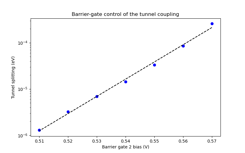
Fig. 17.6.1 Energy splitting between the ground and first excited states of a double quantum dot.
Note the logarithmic scale on the \(y\) axis.
As the barrier gate is decreased from \(0.57\;\mathrm{V}\) to \(0.51\;\mathrm{V}\), the level splitting decreases exponentially, which demonstrates electrostatic control of the tunnel coupling.
Finally, we save the largest tunnel coupling value in a text file for later use in Exchange coupling in a double quantum dot in FD-SOI—Part 1: Perturbation theory.
# Save the largest tunnel splitting in a text file
np.savetxt(path_out/"tunnel_coupling_low_barrier.txt",
    np.array([splittings[0]]))
17.7. Mesh asymmetry and convergence
In this tutorial, we used an offset on plunger gate bias 2 which enabled to symmetrize the double dot wavefunctions despite the presence of numerical asymmetries resulting from the mesh, even for the weakest tunnel coupling.
Below, we show results of an alternative calculation, in which plunger gate bias 2 is optimized in the bias configuration with strong tunnel coupling, instead (i.e., with a barrier gate 2 bias of \(0.57\;\mathrm{V}\)).
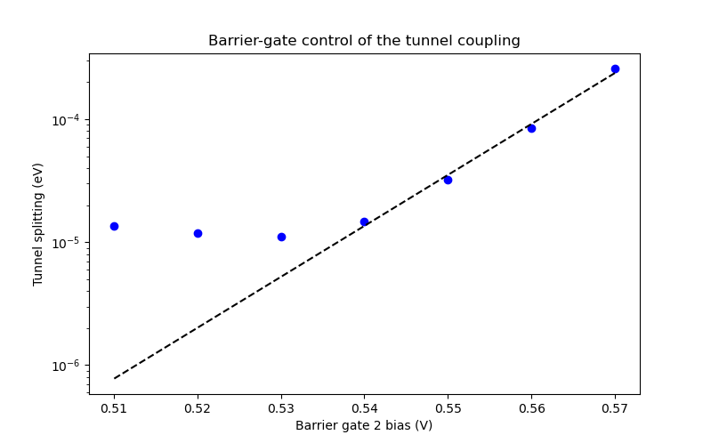
Fig. 17.7.1 Energy splitting between the ground and first excited states of a double quantum dot when the plunger gate 2 bias is optimized in a strong tunneling configuration.
As shown above, as the central barrier gate bias is decreased from its largest value, tunnel coupling first decays exponentially, but then saturates at a value on the order of \(10^{-5}\;\mathrm{eV}\). As explained below, this effect is unphysical.
Saturation of the tunnel coupling occurs because while the plunger gate bias offset found in the strong-tunneling configuration does make the double dot ground state symmetric in this setting, this offset may not be adequate for smaller barrier gate biases. Indeed, because of mesh asymmetry, tuning the central barrier gate may result in slightly asymmetric effects on the confinement potential of each quantum dot, resulting in an effective detuning \(\Delta E\) between the dots. As we reduce the barrier gate bias, we increase the barrier height and thus reduce tunnel coupling \(\Omega\). When \(\Omega\) becomes smaller than \(\Delta E\), the splitting \(E_d \approx \sqrt{\Omega^2+\Delta E^2}\) between the ground and first excited states of the double quantum dot saturates at \(\Delta E\), and the ground state wave function loses its symmetry.
We emphasize that while the plunger gate offsets that enable to symmetrize the wave functions are strongly dependent on the mesh, the tunnel coupling in the optimal bias configuration is much less so. Therefore, similar results for the tunnel coupling as a function of barrier gate bias as those seen in Fig. 17.6.1 would be obtained for finer meshes, provided that tuning of the plunger gate biases is performed separately for each mesh.
17.8. Full code
__copyright__ = "Copyright 2022-2026, Nanoacademic Technologies Inc."

import numpy as np
from pathlib import Path
from matplotlib import pyplot as plt
from qtcad.device import io
from qtcad.device import constants as ct
from qtcad.device.mesh3d import Mesh, SubMesh
from qtcad.device import SubDevice
from qtcad.device.poisson import Solver as PoissonSolver
from qtcad.device.poisson import SolverParams as PoissonSolverParams
from qtcad.device.schrodinger import Solver as SchrodingerSolver
from qtcad.device.schrodinger import SolverParams as SchrodingerSolverParams
from helper.double_dot_fdsoi import get_double_dot_fdsoi

# Set up paths
script_dir = Path(__file__).parent.resolve()
path_mesh = script_dir / "meshes"
path_out = script_dir / "output"

# Load the mesh
scaling = 1e-9
file = path_mesh / "refined_dqdfdsoi.msh"
mesh = Mesh(scaling, file)

# Load the detuning and coupling
path = path_out / "detuning_and_coupling.txt"
detuning, coupling = np.loadtxt(path)

# Define gate biases including the detuning found previously
back_gate_bias = -0.5
barrier_gate_1_bias = 0.5
plunger_gate_1_bias = 0.59
barrier_gate_2_bias = 0.51
plunger_gate_2_bias = 0.59 + detuning
barrier_gate_3_bias = 0.5

# Define the device
dvc = get_double_dot_fdsoi(
    mesh,
    back_gate_bias,
    barrier_gate_1_bias,
    plunger_gate_1_bias,
    barrier_gate_2_bias,
    plunger_gate_2_bias,
    barrier_gate_3_bias,
)

# List of regions forming the double quantum dot region
dot_region_list = ["oxide_dot", "gate_oxide_dot", "buried_oxide_dot", "channel_dot"]

# Configure the non-linear Poisson solver
params_poisson = PoissonSolverParams()
params_poisson.tol = 1e-3  # Convergence threshold (tolerance) for the error
poisson_slv = PoissonSolver(dvc, solver_params=params_poisson)

# Instantiate Schrodinger solver parameters
params_schrod = SchrodingerSolverParams()
params_schrod.tol = 1e-6  # Tolerance on energies in eV

# Load the electric potential from the previous run
phi = io.load(path_out / "tunnel_coupling_final_potential.hdf5", var_name="phi")
dvc.set_potential(phi)

# Create the submesh object for the dot region
submesh = SubMesh(dvc.mesh, dot_region_list)

# Define barrier gate sweep
V_barrier_vec = np.linspace(0.57, 0.51, 7)

# Initialize the energy level array
energy_arr = np.zeros((len(V_barrier_vec), 11))
energy_arr[:, 0] = V_barrier_vec

for idx, V_barrier_2 in enumerate(V_barrier_vec):
    print("=" * 80)
    print("Solving at barrier gate 2 bias: {:.3f} V".format(V_barrier_2))

    # Set barrier height
    dvc.set_applied_potential("barrier_gate_2_bnd", V_barrier_2)

    # Self-consistent solution
    poisson_slv.solve(initialize=False)

    # Calculate the confinement potential from the electric potential
    # The confinement potential is stored in dvc.V
    dvc.set_V_from_phi()

    # Create subdevice for the quantum dots
    subdvc = SubDevice(dvc, submesh)

    # Then instantiate the Schrödinger solver
    schrod_slv = SchrodingerSolver(subdvc, solver_params=params_schrod)

    # Solve Schrödinger's equation
    schrod_slv.solve()

    # Store the solution as an initial guess for the next run
    params_schrod.guess = (subdvc.eigenfunctions, subdvc.energies)

    # Save energy levels
    energy_arr[idx, 1:] = subdvc.energies / ct.e

    np.savetxt(path_out / "tunnel_coupling_energies.txt", energy_arr)

# Calculate the splitting between ground and first excited states
splittings = energy_arr[:, 2] - energy_arr[:, 1]

# Fit a straight line in the log of the splitting
fit = np.polyfit(V_barrier_vec, np.log(splittings), 1)
coeff = np.exp(fit[1])
pref = fit[0]

# Plot the tunnel splittings
fig = plt.figure(figsize=(8, 5))
ax = fig.add_subplot(1, 1, 1)
ax.set_title("Barrier-gate control of the tunnel coupling")
ax.set_xlabel("Barrier gate 2 bias (V)")
ax.set_ylabel("Tunnel splitting (eV)")
ax.set_yscale("log")
ax.plot(V_barrier_vec, splittings, "ob")
ax.plot(
    V_barrier_vec, coeff * np.exp(pref * V_barrier_vec), "--k", label="Exponential fit"
)
plt.show()

# Save the largest tunnel splitting in a text file
np.savetxt(path_out / "tunnel_coupling_low_barrier.txt", np.array([splittings[0]]))