12. Valley coupling (MVEMT)

12.1. Requirements

12.1.1. Software components

12.1.1.1. Basic Python modules

pathlib
numpy
matplotlib

12.1.1.2. Specific modules

qtcad

12.1.2. Python script

qtcad/examples/tutorials/valleycoupling_MVEMT.py

12.1.3. References

12.2. Briefing

In this tutorial we explain how to calculate the valley-coupled eigenenergies and eigenfunctions of a confined conduction-band electron in silicon using a multi-valley effective-mass theory (MVEMT) implemented in QTCAD. The type of confinement we consider in this example is that of a triangular quantum well in the \(z\) direction and harmonic confinement along the \(x\) and \(y\) directions.

It is assumed that the user is familiar with basic Python and has some familiarity with the functionality of the QTCAD code.

The full code may be found at the bottom of this page, or in valleycoupling_MVEMT.py.

12.3. Header

In the header, we import relevant modules.

import pathlib
import numpy as np

from qtcad.device.mesh3d import Mesh
from qtcad.device import constants as ct
from qtcad.device import analysis
from qtcad.device import materials as mt
from qtcad.device import Device

In addition to standard modules already seen in Poisson and Schrödinger simulation of a nanowire quantum dot, the following additional module is used to solve the MVEMT Schrödinger equation.

from qtcad.device.multivalley_EMT import Solver, SolverParams

The multivalley_EMT module defines a multivalley effective mass theory Solver class that can be used to solve the Schrödinger equation derived from the multi-valley effective-mass theory implemented in QTCAD, and described in Multivalley effective-mass theory solver.

12.4. Setting up the device

Now that the relevant modules have been imported, we set up the device to be used in this tutorial. We start by importing the mesh on which our problem will be defined.

# Load mesh from file
script_dir = pathlib.Path(__file__).parent.resolve()
path_mesh = script_dir / "meshes/" / "valleycoupling_MVEMT.msh"
scale = 1e-9
mesh = Mesh(scale, str(path_mesh))

We have used the Mesh constructor to initialize a mesh object from the file located in path_mesh (which gives the absolute path to the relevant mesh file).

Once the mesh is established, we use the Device constructor to initialize a device object from the mesh.

# Create the device from the mesh
d = Device(mesh, conf_carriers="e")

We now have a basic device, d, which we can use to compute valley-splittings and valley-coupled eigenstates of a conduction electron in a simple silicon structure. In a more elaborate simulation, the confinement potential for this structure may be obtained by solving Poisson’s equation. Here, we concentrate on the multi-valley effective mass theory solver, so we will manually specify a simple confinement potential instead.

We start by defining a potential over this device. In this tutorial, we will study a device which has a harmonic potential along the \(x\) and \(y\) directions and a triangular potential along \(z\). We first define a function that describes the smooth part of this potential with

# Potential energy (quadratic in x and y, linear in z + barrier)
def harmonic_potential(x,y,z):
   # # x and y potential
   K = 1e-4 # Spring constant
   V_har = K/2.*(x**2+y**2)
   # # z potential - linear piece
   F = 250e5 # Electric field
   VF = - ct.e * F * z
   return V_har + VF

and set it in the device with

# Set smooth part of the potential
d.set_V(harmonic_potential)

We then discontinuously raise the potential by \(3\textrm{ eV}\) in the barrier region to form a triangular potential with

# Add constant values of the potential in different regions
H = 3 * ct.e # barrier height
d.add_to_V(H, region = 'barrier')

and then raise the entire potential energy by \(1\textrm{ eV}\) across the whole device with

Vmin = 1*ct.e # Potential energy minimum
d.add_to_V(Vmin)

12.5. Material parameters

The basis we are considering for this calculation is made up of the Bloch functions at the conduction band minima of silicon, \(\xi_{\nu}\left(\mathbf{r}\right)\equiv e^{i \mathbf{k}_{\nu}\cdot \mathbf{r}}u_{\nu}\left(\mathbf{r}\right)\) , where \(\nu\) is a valley index, \(\mathbf{k}_{\nu}\) is the location of valley \(\nu\) in the Brillouin zone, and \(u_{\nu}\left(\mathbf{r}\right)\) is the periodic Bloch amplitude at valley \(\nu\) (see Multivalley effective-mass theory solver). Now that the device has been set up, we import three material parameters that are necessary to compute the valley-coupled eigenenergies and eigenfunctions using a multi-valley effective-mass theory calculation:

(1) First, we import the locations of \(\pm z\) valleys within the Brillouin zone, \(\mathbf{k}_{\nu}\) , which are stored in the silicon material file,

# Valley wavevectors
valleys = mt.Si.valleys[4:6]

We also require a description of the Bloch amplitudes, \(u_{\nu}\left(\mathbf{r}\right)\). A Fourier decomposition of these Bloch amplitudes [found in Table I of Saraiva et al. PRB (2011)] is stored in text files found in the directory /device/valleycoupling/bloch/silicon. We specify the path to these files describing the Bloch amplitudes for the \(\pm z\) valleys (with valley_id 'pz' and 'mz', respectively), and specify the silicon lattice constant with

# Bloch amplitudes
qtcad_dir = pathlib.Path(__file__).parent.parent.parent.resolve()
bloch_path = qtcad_dir / "src" / "qtcad" / "device" / "valleycoupling" / "bloch" / "silicon"

a = 5.431e-10 # lattice constant Si
bloch_paths = [bloch_path/"BA_pz_Si.data", bloch_path/"BA_mz_Si.data"]

Finally, we import the effective mass for the \(\pm z\) valleys. These too are stored in the silicon material file

# Effective mass tensors corresponding to valleys.
me_inv = mt.Si.Me_inv_valley[4:6]

The reason why we only import the material parameters for the \(\pm z\) valleys is that the potential we have set up in the previous section describes strong confinement in the \(z\) direction (relative to the \(x\) and \(y\)) directions. Therefore, we expect the \(\pm z\) valleys to be the ground states and to be split from the other valleys by an amount that depends on their relative effective masses along the \(z\) direction.

12.6. Solving the (MVEMT) Schrödinger equation

Before defining the MVEMT solver, we define its parameters using a SolverParams object.

# Compute valley coupling (using form-factor approximation)
params = SolverParams()
params.num_states = 2
params.approx = "ff"

Here, we have set the number of states to account for in the MVEMT to 2, meaning that we will only be solving for the two lowest valley–orbit states. In addition, we have set the approx solver parameter to "ff". Indeed, this solver parameter allows for the application of approximations when handling the Bloch amplitudes. The default values for approx is 'ff' which enforces the form-factor approximation. For more information on the form-factor approximation, see the supplemental material for [GHCJ+16]. Other possibilities for the value of approx are the envelope-function approximation using approx = 'envelope', and no approximations using approx = None. The form-factor and envelope-function approximations allow for the calculation to be sped up while sacrificing some accuracy for the final result.

Once the optional solver parameters are defined, we instantiate a MVEMT Solver object with

vc = Solver(d, valleys, bloch_paths, me_inv, a, solver_params=params)

using as arguments the device d, the valley positions valleys, the paths to the files giving the Bloch amplitude Fourier decomposition bloch_paths, the inverse effective mass tensors me_inv, the lattice constant a, and the solver parameters params.

Now that the MVEMT Solver object has been initialized, we run the solve method to obtain the eigenenergies and eigenfunctions

vc.solve()

Here, the solve method will compute the two lowest energy eigenfunctions. The solve method stores the eigenenergies and eigenfunctions in the device d, in the energies and eigenfunctions attributes. The energies can be output by running

print("Valley-coupled eigenenergies (eV):")
print(d.energies/ct.e)

The output will contain the two lowest energies in the spectrum:

Valley-coupled eigenenergies (eV):
[0.89028668 0.89076318]

The difference in these two energies represents the ground-state valley-splitting in the subspace of the \(\pm z\) valleys.

12.7. Visualization

To visualize the eigenfunctions, we plot the associated density. The eigenfunctions are stored in the device attribute d.eigenfunctions. The dimensions of this attribute can be obtained via

# Plot functions
print('Dimensions of eigenfunctions:')
print(d.eigenfunctions.shape)

which will output the dimensions in a tuple:

Dimensions of eigenfunctions:
(6030, 2, 2)

The first index goes over all the nodes in the domain (position index), the second identifies the eigenstate (ground state, first excited state, etc.), and the third index goes over the basis (\(+z\) and \(-z\) valley contributions). Here we use the built-in plotting functionality of the analysis module to plot the \(+z\) and \(-z\) contributions to the ground state

# Plot +z and -z valley components
analysis.plot_slices(mesh,np.absolute(d.eigenfunctions[:,0,0])**2,
    title="Ground state | +z valley")
analysis.plot_slices(mesh,np.absolute(d.eigenfunctions[:,0,1])**2,
    title="Ground state | -z valley")

The outputs (for the \(+z\) and \(-z\) contributions respectively) are shown below.

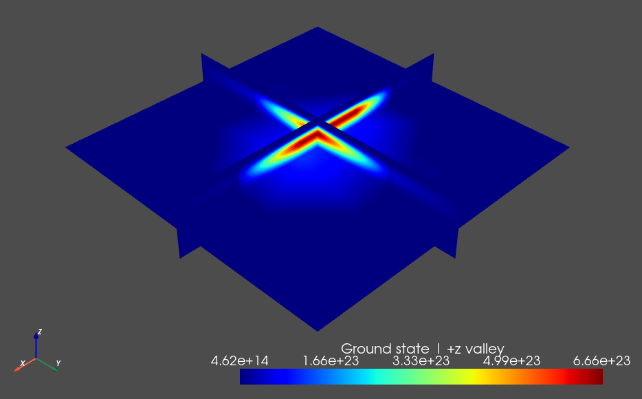
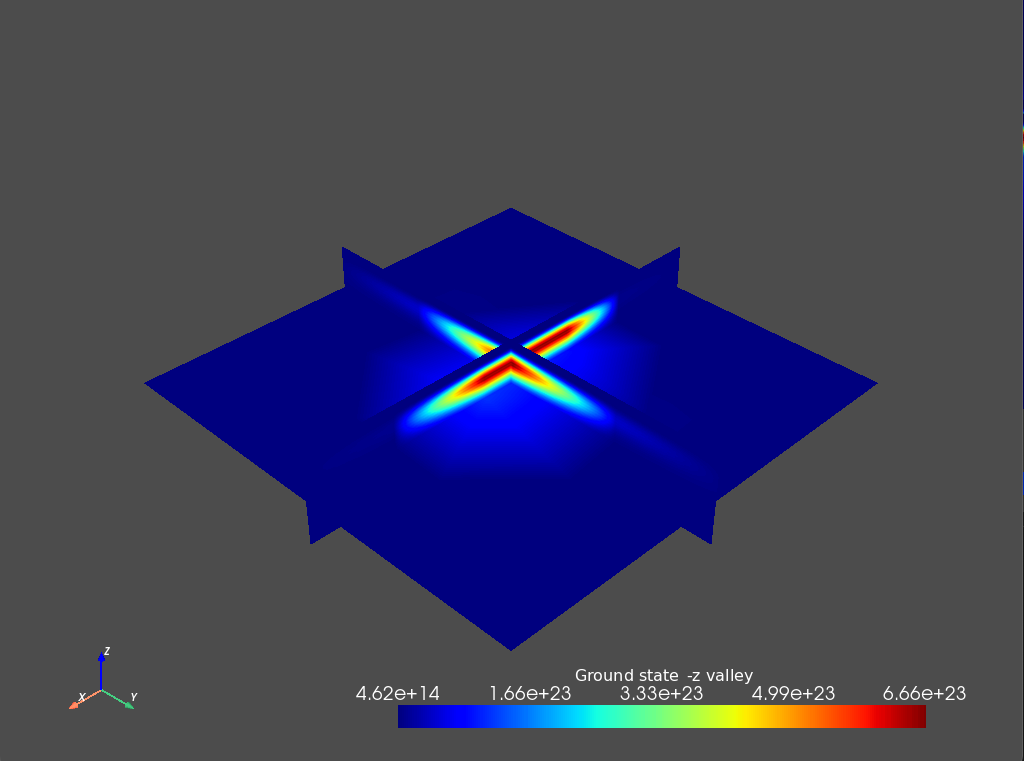
+z Valley contribution to the ground state — Fig. 12.7.1 \(+z`\) Valley contribution to the ground state

From these plots we see that the ground state has an almost equal (up to some numerical error) contribution from each valley, as is expected from symmetry considerations.

In the next tutorial (Electric dipole spin resonance—Dynamics), we will add a slanting magnetic field to study electric-dipole spin resonance in a gated quantum dot system.

12.8. Full code

__copyright__ = "Copyright 2024, Nanoacademic Technologies Inc."

import pathlib
import numpy as np
from qtcad.device.mesh3d import Mesh
from qtcad.device import constants as ct
from qtcad.device import analysis
from qtcad.device import materials as mt
from qtcad.device import Device

from qtcad.device.multivalley_EMT import Solver, SolverParams

# Load mesh from file
script_dir = pathlib.Path(__file__).parent.resolve()
path_mesh = script_dir / "meshes/" / "valleycoupling_MVEMT.msh"
scale = 1e-9
mesh = Mesh(scale, str(path_mesh))

# Create the device from the mesh
d = Device(mesh, conf_carriers="e")

# Potential energy (quadratic in x and y, linear in z + barrier)
def harmonic_potential(x,y,z):
   # # x and y potential
   K = 1e-4 # Spring constant
   V_har = K/2.*(x**2+y**2)
   # # z potential - linear piece
   F = 250e5 # Electric field
   VF = - ct.e * F * z
   return V_har + VF

# Set smooth part of the potential
d.set_V(harmonic_potential)

# Add constant values of the potential in different regions
H = 3 * ct.e # barrier height
d.add_to_V(H, region = 'barrier')

Vmin = 1*ct.e # Potential energy minimum
d.add_to_V(Vmin)

# Valley wavevectors 
valleys = mt.Si.valleys[4:6]

# Bloch amplitudes
qtcad_dir = pathlib.Path(__file__).parent.parent.parent.resolve() 
bloch_path = qtcad_dir / "src" / "qtcad" / "device" / "valleycoupling" / "bloch" / "silicon"

a = 5.431e-10 # lattice constant Si
bloch_paths = [bloch_path/"BA_pz_Si.data", bloch_path/"BA_mz_Si.data"]

# Effective mass tensors corresponding to valleys.
me_inv = mt.Si.Me_inv_valley[4:6]

# Compute valley coupling (using form-factor approximation)
params = SolverParams()
params.num_states = 2
params.approx = "ff"

vc = Solver(d, valleys, bloch_paths, me_inv, a, solver_params=params)

vc.solve()

print("Valley-coupled eigenenergies (eV):")
print(d.energies/ct.e)

# Plot functions
print('Dimensions of eigenfunctions:')
print(d.eigenfunctions.shape)

# Plot +z and -z valley components
analysis.plot_slices(mesh,np.absolute(d.eigenfunctions[:,0,0])**2,
    title="Ground state | +z valley")
analysis.plot_slices(mesh,np.absolute(d.eigenfunctions[:,0,1])**2,
    title="Ground state | -z valley")