5. Multivalley effective-mass theory solver

Differential equation

We consider a material with conduction-band minima (valleys) located at \(\mathbf k_\nu\), with \(\nu\) being the valley index. Within multivalley effective-mass theory, we approximate the conduction-electron wavefunctions as [GJN+15, SN76]

(5.1)\[\psi(\mathbf r) = \sum_\nu F_\nu(\mathbf r) \xi_{\nu} (\mathbf r),\]

where the sum is over all degenerate valleys \(\nu\). In Eq. (5.1), we have introduced \(F_\nu(\mathbf r)\), the envelope function for valley \(\nu\), and \(\xi_\nu(\mathbf r)\equiv u_\nu(\mathbf r)\mathrm e^{i\mathbf k_\nu\cdot\mathbf r}\), the Bloch function evaluated at the \(\nu\)-th conduction band minimum, with \(u_\nu (\mathbf r)\) being the lattice-periodic Bloch amplitude of this state.

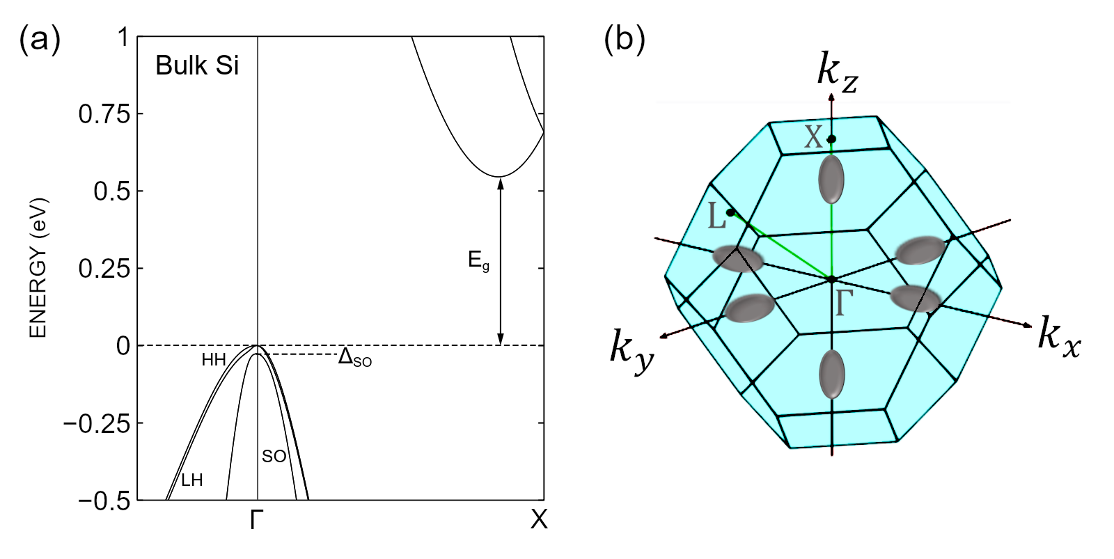
Fig. 5.1 Degenerate conduction-band minima (valleys) in silicon. (a) Band structure of silicon (Si). (b) First Brillouin zone of silicon. The ellipsoids are equipotential surfaces of the conduction band of silicon near its six equivalent minima located away from the \(\Gamma\) point along the \(\pm \mathbf{\hat x}\), \(\pm \mathbf{\hat y}\), and \(\pm \mathbf{\hat z}\) directions, at roughly 85 % of the distance between the \(\Gamma\) point and the zone boundary (only the X point is shown above). The band structure in (a) was calculated using Nanoacademic’s atomistic simulation software NanoDCAL (see, e.g., the NanoDCAL tutorial on Spin–orbit interaction). Similar calculations can also be done with RESCU and RESCU+. The band structure was calculated using the local density approximation (LDA), which correctly predicts numerous properties of crystals but underestimates band gaps.

Assuming that the lengthscale for variations of the envelope functions is much larger than the lengthscale for variations of the Bloch functions (which is commensurate with the lattice constant), a set of coupled Schrödinger equations may be written as

(5.2)\[-\frac{\hbar^2}2\nabla\cdot\mathbf M^{-1}_\nu\cdot \nabla F_\nu(\mathbf r) + \sum_{\nu'} V^\mathrm{VO}_{\nu\nu'}(\mathbf r) F_{\nu'}(\mathbf r) = E F_\nu(\mathbf r),\]

where \(\mathbf M_\nu^{-1}\) is the effective mass tensor for valley \(\nu\). Remark that we have one equation for each valley, and that these equations are coupled by the second term on the left-hand side of Eq. (5.2), which contains

(5.3)\[V^\mathrm{VO}_{\nu\nu'}(\mathbf r) = \frac1{|\Omega|} \int_{\Omega_\mathbf r} d\boldsymbol \rho \; \xi^\ast_\nu(\mathbf r + \boldsymbol \rho) V_\mathrm{conf}(\mathbf r + \boldsymbol \rho) \xi_{\nu'}(\mathbf r + \boldsymbol \rho),\]

where \(\Omega_{\mathbf r}\) is the lattice unit cell located at position \(\mathbf r\), and \(|\Omega_{\mathbf r}|=|\Omega|\;\forall\;\mathbf r\) is the unit cell volume (which is the same for all \(\mathbf r\) for a homogeneous semiconductor).

The quantity \(V^\mathrm{VO}_{\nu\nu'}(\mathbf r)\) introduced in Eq. (5.3) describes the impact of the confinement potential on the electronic structure of the device. If the confinement potential varies significantly over the lattice spacing, the term \(V^\mathrm{VO}_{\nu\nu'}(\mathbf r)\) in Eq. (5.3) gives rise to significant coupling between the valleys \(\nu\) and \(\nu'\) (valley–orbit coupling). In contrast, if the confinement potential varies negligibly over the lattice spacing, no significant coupling between the valleys arises due to the orthonormality of the Bloch functions, resulting in \(V^\mathrm{VO}_{\nu\nu'}(\mathbf r)\approx V_\mathrm{conf}(\mathbf r)\delta_{\nu\nu'}\).

To calculate the valley–orbit coupling term defined in Eq. (5.3), it is useful to write the Bloch amplitudes as a Fourier decomposition:

(5.4)\[u_\nu(\mathbf r) = \sum_{\mathbf G} A_{\mathbf G}^\nu \mathrm e^{i\mathbf G\cdot\mathbf r},\]

where \(A_\mathbf G^\nu\) is the Fourier component of the Bloch amplitude associated with the reciprocal lattice vector \(\mathbf G\). These Fourier components may be calculated using density-functional theory (e.g. with RESCU+). In QTCAD, it is possible to import the Fourier components of Bloch amplitudes from text files. In particular, it is possible to import Fourier components of the silicon Bloch amplitudes calculated in [SCalderonC+11]; these Fourier components are stored in qtcad/device/valleycoupling/bloch/silicon.

More practical information on how to use the multi-valley effective mass theory solver and the bloch_tools module may be found in the Valley coupling (MVEMT) tutorial.

Relevant device attributes

Parameter	Symbol	QTCAD name	Unit	Default	Setter
Confinement potential	\(V\)	V	J	0	set_V_from_phi, set_V
External conf. potential	\(V_\mathrm{ext}\)	Vext	J	0	set_Vext

Note

The total confinement potential \(V_\mathrm{conf} (\mathbf r)\) employed by the multivalley effective mass theory solver is given by \(V_\mathrm{conf} (\mathbf r) = V(\mathbf r)+V_\mathrm{ext}(\mathbf r)\).

Boundary conditions

The boundary conditions for the multi-valley effective mass theory solver are the same as for the regular Schrödinger solvers. These boundary conditions are described in Boundary conditions.