10. Transport in the Coulomb blockade regime
In this section, we describe the basic equations implemented in QTCAD to model
transport under strong quantum confinement (such as through a quantum dot).
The most important effect that is captured by the QTCAD
junction simulator is the
Coulomb blockade. Through QTCAD transport simulations, it is possible
to calculate Coulomb peaks and charge-stability diagrams, which are used
experimentally to demonstrate the single-electron regime.
The junction concept
Fig. 10.1 illustrates the junction concept, which is implemented
in the Junction class of the QTCAD
transport simulator.
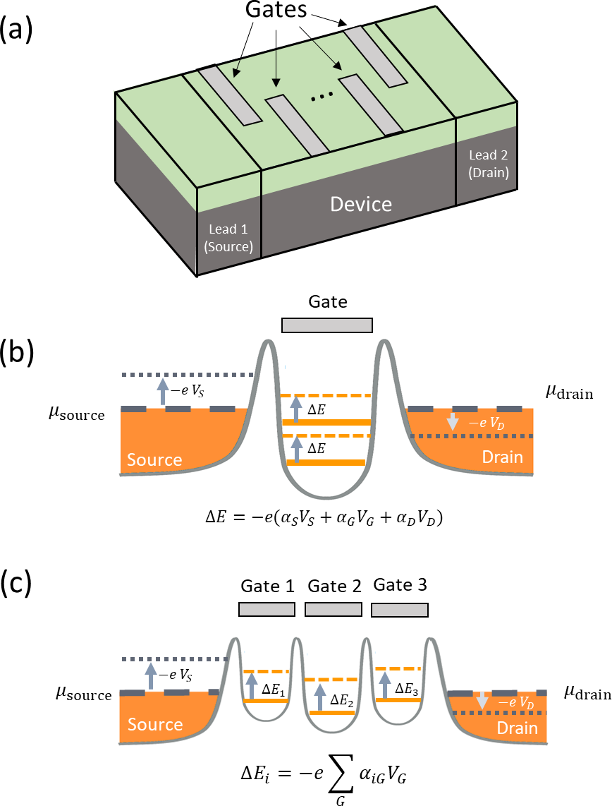
Fig. 10.1 The junction concept. (a) Real-space schematic representation of a quantum dot system (device) in contact with two leads: lead 1 (the source) and lead 2 (the drain). The device may include a certain number of arbitrarily-shaped gates used to control the quantum dot confinement potential landscape. (b) Energy-space representation of the same structure in the case of a single quantum dot with a single control gate. The source, drain, and dot chemical potentials can be rigidly shifted by applying phenomenological biases, accounting for lever arms calculated using QTCAD, which accurately account for realistic device geometry. (c) Generalization to a multiple-dot system (here, a triple quantum dot). The single-electron energy levels of the quantum-dot system are assumed to depend linearly on the control gate biases with cross-capacitive effects being accounted for through the lever arm matrix.
A junction consists of a
Device or
SubDevice object connected to two
Lead objects, as illustrated
schematically in real space in Fig. 10.1 (a). The device
is always modeled explicitly in real space. In contrast, the leads may
either be modeled phenomenologically using the
Lead class, in which case no explicit
geometric representation is considered, or explicitly using the
WKBLead class, in which case
the leads are explicitly associated with certain physical regions of a
Device object.
The electrostatics and energy-level structure of the source, drain and dot may
be calculated with the QTCAD Device simulator, accounting
for full device geometry. Once stored inside a
Junction object,
these energy levels may be shifted by phenomenological gate
potentials, accounting for lever arms that are either input from experimental
data, or calculated from the device geometry using QTCAD’s Poisson and
Schrödinger solvers (see Lever arm theory, Calculating the lever arm of a quantum dot,
and Quantum transport—Charge stability diagram of a double quantum dot).
This approach enables to save time because it avoids having to solve the
Poisson and Schrödinger equations every time the gate potential is changed.
Fundamental tunneling Hamiltonian
In QTCAD’s transport solver, we consider a many-body description of the device, including Coulomb interactions between electrons. In addition, we consider that coupling between the device and the leads arises from tunneling events. We thus use the following Hamiltonian for the device and leads in the Fock basis corresponding to single-electron eigenfunctions of the source, drain, and leads:
In Eq. (10.1), the first line corresponds to the many-body Hamiltonian introduced in Eq. (8.5), in which \(\epsilon_{i\sigma}\) is the energy of the single-electron eigenstate with orbital index \(i\) and degeneracy index \(\sigma\) (arising from, e.g., spin or valley), and \(V_{ijlk}\) represents matrix elements of the Coulomb interaction defined in Eq. (8.6). The first term of the second line is the free Hamiltonian of the source and drain, with \(\epsilon_{\mathbf kL}\) the energy of a lead \(L\in \{\textrm{S}, \textrm{D}\}\) (source or drain) eigenstate with wave vector \(\mathbf k\). Finally, the last term of the equation captures tunneling between the device and the leads, with \(t_{\mathbf kL,i\sigma}\) being the tunneling matrix element between \((i\sigma)\) and \(\mathbf k\) single-electron eigenstates of the device and lead \(L\), respectively.
The sequential tunneling master equation
In the QTCAD transport simulator, the approach is
to first diagonalize the device Hamiltonian using the exact diagonalization
technique introduced in Many-body solver, and then treat coupling to
the leads as a weak perturbation.
Within the sequential tunneling regime, we model transport through the device using the master equation [BF04]
where we have assumed steady-state conditions. In (10.2), we have introduced the indices \(n\) and \(m\), which run over all the many-body eigenstates of the device. In addition, we have introduced the occupation probability \(p_m\) of state \(m\) (note that occupation probabilities are subject to the condition \(\sum_m p_m=1\)) and the total transition rates
from state \(n\) to state \(m\), where \(\Gamma^{\textrm S(\textrm D)}_{n\rightarrow m}\) is the contribution to the transition rate induced by the source (drain) lead.
The tunneling Hamiltonian introduced in Eq. (10.1) may cause two types of transitions between many-body eigenstates. Representing the \(\alpha\)-th many-body eigenstate within the \(N\)-electron subspace as \(|\alpha_N\rangle\), tunneling may lead to transitions of the form \(|\alpha_N\rangle\rightarrow |\beta_{N+1}\rangle\) (the device absorbs an electron from the lead) or \(|\alpha_N\rangle\rightarrow |\beta_{N-1}\rangle\) (the device releases an electron into the lead). The rates for these transitions are given by Fermi’s golden rule:
where \(L\;\in\;\{\textrm S, \textrm D\}\) is the lead index (source or drain), \(\mu\) and \(\nu\) are collective indices that simultaneously label the orbital-state and degeneracy indices of the single-electron basis states (i.e., \(\mu\to i,\sigma\); \(\nu \to j,\sigma'\)), \(E^N_\alpha\) is the energy of the many-body eigenstate \(|\alpha_N\rangle\), \(\mu_L\) is the chemical potential of the lead \(L\), and \(n_F(x)\) is the Fermi–Dirac distribution
Importantly, in Eq. (10.4), we have introduced the broadening function
where \(\mathbf k_L\) labels single-electron eigenstates of lead \(L\).
As will be seen below, there are two ways in which the broadening function may be evaluated in QTCAD:
through a featureless approximation,
using the WKB approximation.
Broadening function: featureless approximation
In the featureless approximation, the broadening function
\(\Gamma^L_{\mu\nu}(E)\) is simply taken to be a constant independent
of \(E\), \(\mu\), and \(\nu\) for each lead. By default,
this constant is \(1\;\textrm{Hz}\) in QTCAD, but may be modified
to arbitrary values through the
set_source_broad_func
and
set_drain_broad_func
methods of the
Junction class.
See Calculating the charge-stability diagram of a quantum dot for an example of transport simulation in which these methods are used.
Broadening function: WKB calculation
The Wentzel–Kramers–Brillouin (WKB) approximation is a famous method used in the calculation of one-dimensional quantum tunneling problems.
To use the WKB approximation to calculate the broadening function, we make the following assumptions:
The Schrödinger equation of the relevant lead is separable in the \(x\), \(y\), and \(z\) directions: the lead potential is given by \(V_L(x,y,z) = V^L_x(x) + V^L_y(y) + V^L_z(z)\).
The source, device, and drain are aligned along a single Cartesian axis; in this theory section, we choose this axis to be the \(x\) axis.
Within the relevant lead, there is confinement along the \(y\) and \(z\) directions, leading to lead subbands associated with quantum numbers \(n_y\) and \(n_z\), respectively.
A single effective mass \(m^\ast\) can be defined in the transport direction.
A continuum (density-of-states) approximation may be taken for the lead eigenstates along \(x\).
Under these assumptions, the broadening function is given by
where \(E_{n_y}\) and \(E_{n_z}\) are the eigenenergies of the lead Schrödinger equations along the transverse directions \(y\) and \(z\), and \(\ell\) is the length of the lead in the \(x\) direction.
The tunneling matrix elements \(t_{n_y,n_z,\mu}(E)\) entering Eq. (10.7) are given by the transition matrix elements [Rei95]
where \(\psi_{\textrm D}(\mathbf{r})\) is a device single-particle envelope function and \(\psi_L(\mathbf{r}) = \psi^{WKB}_L(x)\psi^{y}_L(y)\psi^{z}_L(z)\) is a lead wave function (recall the separability assumption). As illustrated below, we have also introduced the barrier height \(V_0\), the quantum dot potential \(V_{\textrm D}(\mathbf{r})\), and the barrier position \(x_1\). In the figure below, we have also introduced \(V^{\textrm D}_x(x)\), a linecut of \(V_{\textrm D}(\mathbf{r})\) along the \(x\) direction.
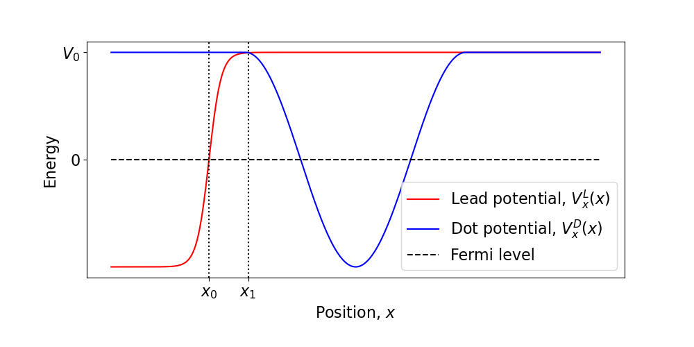
Fig. 10.2 Potentials involved in the calculation of the transition matrix elements.
The quantum dot wave function is easily calculated by numerically solving Schrödinger’s equation in the dot region (see, e.g., Simulating bound states in a quantum dot using the Poisson and Schrödinger solvers). In contrast, the lead wave function along \(x\) is obtained analytically using the WKB approximation
where \(D\) is a normalization constant and
In the above equations, we have introduced \(\epsilon = E - E_{n_y} - E_{n_z}\), the energy of the lead electron reserved for motion along \(x\). We have also introduced \(x_0\), the classical turning point of the lead potential.
Note that in Eq. (10.8), we have assumed that the quantum dot wave function is negligible for \(x<x_1\). This is a crucial approximation since in QTCAD, quantum dot wave functions are calculated within dot regions whose boundaries loosely coincide with barrier locations.
Note
In QTCAD, \(x_1\) is chosen automatically as the edge of the
SubDevice representing the quantum
system (SubDevice over which the
Schrödinger equation is solved to find bound states) along the transport
direction.
For an example, see see Quantum transport—WKB approximation.
Note
The WKB feature is currently limited to single-valley electron calculations. In other words, it is currently not possible to use the WKB feature in combination with the Schrödinger solver for holes, or with the multi-valley effective-mass theory solver.
Sequential tunneling current
The charge current associated with electrons entering the device from the source is
Also, introducing the charge current \(I^\textrm D\) associated with electrons entering the device from the drain, we have
due to charge conservation.
Therefore, the current flowing through the device can easily be calculated from the occupation probabilities (obtained by solving the master equation) and the transition rates introduced above.
Particle addition spectrum
When the source–drain bias is sufficiently small, the quantum dot system is approximately at thermodynamic equilibrium with the leads. Since we are ultimately interested in the charge stability diagram of the quantum dot system, a central quantity of interest is the total particle number \(N=\sum_i n_i\), with \(n_i\) the number of particles in orbital \(i\) introduced in Eq. (8.16). At thermal equilibrium with a heat bath at constant temperature \(T\) and chemical equilibrium with leads at chemical potential \(\mu\), the average particle number is
where we have introduced the grand partition function
Transitions in the total particle number are associated with peaks in the particle addition spectrum defined by [HFJ+17]
Computing this particle addition spectrum as a function of gate bias configurations gives diagrams in which non-zero values indicate configurations that allow the total particle number to change as a function of source and drain chemical potentials, and thus for the steady-state current flowing through the quantum dot system to change. In many cases, this can allow to identify transitions in charge stability diagrams more efficiently (see, e.g., the Quantum transport—Charge stability diagram of a double quantum dot tutorial).