2. Quantum transport—WKB approximation
2.1. Requirements
2.1.1. Software components
qtcad
2.1.2. Python script
qtcad/examples/tutorials/WKB_current.py
2.1.3. References
Warning
This module will be deprecated in QTCAD 2.3. Please use the recommended workflow described in Poisson–NEGF–Master-equation simulations of an FD-SOI field-effect transistor with a single quantum dot.
2.2. Briefing
In this tutorial, we will again demonstrate how to perform a quantum transport calculation. This calculation will be similar to the one demonstrated in Quantum transport—Master equation, however it will include a method for getting a quantitative estimate of the values of the currents being investigated. This method is based on the WKB approximation.
2.3. Setting up the device
2.3.1. Header
Here we import the modules from Schrödinger equation for a quantum dot and,
similarly to the previous tutorial (Quantum transport—Master equation), relevant
classes and functions from the
transport package.
import numpy as np
from matplotlib import pyplot as plt
import pathlib
from progress.bar import ChargingBar as Bar

from qtcad.device.mesh3d import Mesh, SubMesh
from qtcad.device import constants as ct
from qtcad.device import materials as mt
from qtcad.device import Device, SubDevice
from qtcad.device.schrodinger import Solver
from qtcad.device.schrodinger import SolverParams as SingleBodySolverParams
from qtcad.device.many_body import SolverParams as ManyBodySolverParams

from qtcad.transport.junction import Junction
from qtcad.transport.lead import WKBLead
from qtcad.transport.mastereq import seq_tunnel_curr
From the transport module we have:
Junction: Class that contains all information about the transport system, i.e. the two leads (source and drain), and the quantum-dot system.
WKBLead: Class that allows to define leads whose wavefunctions are estimated using the WKB approximation
seq_tunnel_curr: Function to compute transport properties
2.3.2. Load data and device setup
This section is identical to the
example creating_dot.py presented in Schrödinger equation for a quantum dot, in which more
details may be found. In short, we set up a device which has a lead, a quantum
dot, and another lead. There are also potential barriers
between each lead and the dot.
# Paths to mesh file and output files
script_dir = pathlib.Path(__file__).parent.resolve()
path_mesh = script_dir / "meshes/" / "lead_dot_lead.msh"
scalingFactor = 1e-9
mesh = Mesh(scalingFactor, str(path_mesh))

# Create the device from the mesh
d = Device(mesh, conf_carriers="e")

d.new_region('dot', mt.GaAs)
d.new_region('lead', mt.GaAs)
d.new_region('lead2', mt.GaAs)
d.new_region('barrier', mt.GaAs)
d.new_region('barrier2', mt.GaAs)

# Global nodes
x = mesh.glob_nodes[:, 0]
y = mesh.glob_nodes[:, 1]
z = mesh.glob_nodes[:, 2]

# Potential along y and z
# Position of the harmonic oscillator minimum
y0 = 0
z0 = 0
Ky = 2e-7 # Parabolic in y
Kz = 1e-4 # Parabolic in z
Vy = Ky/2.*(y-y0)**2
Vz = Kz/2. * (z-z0)**2
# Set the potential energy
d.set_V(Vy + Vz)

# Add the potential energy along x
d.add_to_V(12e-3 * ct.e, region='barrier')
d.add_to_V(12e-3 * ct.e, region='barrier2')
d.add_to_V(-10e-3 * ct.e, region='lead')
d.add_to_V(-10e-3 * ct.e, region='lead2')
d.add_to_V(-1e-2 * ct.e)

# Create submesh
dotmesh = SubMesh(d.mesh, ['dot', 'barrier', 'barrier2'])
# Create subdevice
dot = SubDevice(d, dotmesh)
# Solve the Schrodinger equation.
# Configure the Schrödinger solver
params_schrod = SingleBodySolverParams()
params_schrod.num_states = 10 # Number of energy levels to consider
params_schrod.tol = 1e-9 # Set the tolerance for convergence

# Create solver
s = Solver(dot, solver_params=params_schrod)
s.solve() # solve
2.3.3. Initializing lead objects
Now that the dot has been initialized and its eigenenergies solved for, we focus on the leads. We initialize two lead objects: a left lead (source) and a right lead (drain). Currently, QTCAD only supports one type of lead where the eigenstates are explicitly modeled; this is based on the WKB approximation. Since the WKB approximation only works for problems with one spatial dimension, we must reduce the Schrödinger equation for the leads from three to one dimension. To achieve this dimensional reduction, we rely on an approximation: we will assume that the potential for the leads is separable, i.e.
The potentials \(V_x \left( x \right)\), \(V_y \left( y \right)\),
and \(V_z \left( z \right)\) are determined by
taking three different linecuts of the full (3D) potential. Each of
these linecuts will have a fixed value for two out of the three
coordinates (\(x\), \(y\), and \(z`\)). The fixed values are given
as a 3-tuple by the user and in this tutorial are stored in L_intersection
and R_intersection for the left and right leads respectively. This tuple
is represented schematically in the figure below. The linecuts are taken
along the dashed blue lines which are determined by the tuple (x0, y0,
z0).
Fig. 2.3.1 Intersection point
Along the direction where we expect current, the wavefunction will be approximated using the WKB approximation, and along the other two direction, the one-dimensional Schrödinger equation will be solved. There is therefore a baked-in assumption in the procedure that the lead states are extended (propagating) only along one Cartesian coordinate, while they are fully confined along the other two. We note that in this specific example the separability approximation is exact by construction.
Along with the tuple L_intersection (or R_intersection), the
WKBLead constructor also takes other inputs:
the device
da list of strings that contains the tags of the regions where the dot is defined
a list of strings that contains the tags of the regions where the lead is defined
the intersection point defining the linecuts (see figure above)
the direction along which the WKB approximation will be applied, i.e. the transport direction (the possible inputs are
'x','y', or'z'). In this example, this direction is'x'.the effective mass of electrons in both leads; this must be a scalar.
the number of confined one-dimensional states to consider in the first transverse direction (in this case, the
'y'direction)the number of confined one-dimensional states to consider in the second transverse direction (in this case, the
'z'direction). We note that the “first” and “second” transverse direction are determined by taking a cyclic permutation of'x','y','z', starting from the transport direction E.g. if the transport direction is'y', the first and second transverse direction will be'z'and'x'respectively.the resolution (number of sample points) along the linecuts
a list of tags for any additional regions in which the lead potential can extend beyond the quantum-dot region. In this example, the wavefunction inside the first lead (
'lead'tag) may extend into the second lead ('lead2'tag) through the quantum-dot region, and vice-versa. This is only relevant to normalize the lead wavefunction in cases in which it significantly extends beyond the dot region into the other lead.
# Take linecuts to define lead potential
# Length of dot region
L_dot = 200 * scalingFactor
# Length of left lead
L_lead1 = 50 * scalingFactor
# Length of right lead
L_lead2 = 50 * scalingFactor

x0 = L_lead1 - 10*scalingFactor
x0R = L_lead1 + L_dot + 10*scalingFactor

L_intersection = (x0, y0, z0)
R_intersection = (x0R, y0, z0)

# Define the leads.
mass = 1 / mt.GaAs.Me_inv[0,0]
R_lead = WKBLead(d, ['dot', 'barrier', 'barrier2'], R_intersection, 'x', ['lead2'],
   mass=mass, n1=1, n2=1, extra_region=['lead'])
L_lead = WKBLead(d, ['dot', 'barrier', 'barrier2'], L_intersection, 'x', ['lead'],
   mass=mass, n1=1, n2=1, extra_region=['lead2'])
Note
The \(x_1\) point which defines the boundary between the dot region and
the lead region (see Broadening function: WKB calculation) is determined automatically as the
maximal (minimal) coordinate in the dot region (defined by dot) along
the transport direction for the right (left) lead, R_lead (L_lead).
The WKBLead objects also have built-in plotting functionalities that
can be used to plot the lead wavefunction and the potential along the
different linecuts mentioned above. The plot_lead_wf method takes as
input:
the total energy of the state that is to be plotted along (in this case we use a test value
Etest; recall that the zero of energy is set to be the chemical potential throughout the device at equilibrium)the state index (quantum number) associated with the confinement along each perpendicular direction (
'y'and'z'in this example)the directions along which we wish the wavefunction to be plotted (here we have chosen all three directions
'x','y', and'z')
# Plot lead wavefunctions for a given energy
Etest = 5e-3*ct.e
R_lead.plot_lead_wf(Etest, 0, 0, 'x', 'y', 'z')
L_lead.plot_lead_wf(Etest, 0, 0, 'x', 'y', 'z')
The plots produced are:
Fig. 2.3.2 Wave function and confinement potential for the right lead.
Fig. 2.3.3 Wave function and confinement potential for the left lead.
where the dashed lines are for the electron density and the solid line for the potential. We can see from these plots that the electrons are bound in the \(y\) and \(z\) directions, but are extended in the \(x\) direction.
Note
The plot_lead_wf method also has an optional argument path which
is None by default.
If a path is given, the plot will be saved to the specified location.
Otherwise, if None, the plot will be displayed on the screen.
2.3.4. Initializing the junction object
Once the leads and dot (device) have been initialized, we can initialize a junction object through the following interface
# Define the junction (left lead - dot - right lead)
many_body_solver_params = ManyBodySolverParams()
many_body_solver_params.num_states = 1
many_body_solver_params.n_degen = 2
junc = Junction(dot, L_lead, R_lead,
   many_body_solver_params=many_body_solver_params)
dot:
Junctionkeeps a copy of the device object representing the dotL_lead and R_lead: The left (source) and right (drain) leads must be given to the
Junctionn_degen: Parameter to specify the degeneracy of the single particle states. Can be used to account for e.g. spin or valley degeneracy. Set to
n_degen = 2in this example to account for spin.num_states: Number of one-particle eigenstates to be included in the many-body basis set. The Fock-space dimension in the following many-body simulation is thus 2^(num_states*spin)
The initialization procedure may take a while since the program will set
up the many-body Hamiltonian and diagonalize it. For a junction jc,
the many-body eigenenergies can be extracted via
jc.get_all_eig_energies()
After initialization one may still be able to set certain parameters through Junction-class setters, such as
jc.set_temperature(1)   # set temperature in Kelvin
jc.setVg(0.1)  # set gate voltage in volts
jc.setVs(0.1)  # set source voltage in volts
jc.setVd(0.1)  # set drain voltage in volts
The source-to-drain voltages are assumed to rigidly shift the chemical potentials of corresponding reservoirs, and applying a gate voltage effectively shifts the entire energy spectrum of the device by \(-e V_g\), corresponding to an ideal lever arm \(\alpha=1\).
Note that the electrostatics is not recalculated when we manually set
these potential parameters. However, the actual lever arm for a given
device geometry may be accounted for by setting the keyword argument
alpha of the setVg method to the chosen value (different from
the default value of 1). The single-particle eigenenergies are then
shifted by \(-e\alpha V_g\) when applying a gate potential \(V_g\).
The lever arm \(\alpha\) may easily be found by finding the single-particle
eigenenergies as a function of \(e V_g\), and fitting the result to a
straight line. The slope of this line then gives \(-\alpha\).
Note
We can also use the junction, jc, to compute tunneling matrix elements
between the leads and the dot.
This is done by calling the
get_tunneling_mat_elem
method and passing the
energy of the transition, an integer representing the index of the dot state
involved in the transition, a tuple of two integers representing the indices
of the lead state along the confined directions involved in the transition,
and an index (1 or 2) to specify if we are considering tunneling from the
first or second lead.
For example, we could compute the tunneling matrix element for a transition
at Etest from the ground subband of the left lead to the quantum-dot
ground state using the following line of code:
jc.get_tunneling_mat_elem(Etest, 0, (0, 0), 1)
2.4. Transport calculation
2.4.1. WKB approximation - Coulomb peaks
To calculate transport currents and statistical distribution we invoke
the seq_tunnel_curr function
Il, Ir, prob = seq_tunnel_curr(junc)
Il: charge current from source
Ir: charge current from drain. The relationship
Il+Ir=0 should be respected.prob: occupation probability for each many-body state in the stationary (steady-state) regime.
In this tutorial we will first produce Coulomb peaks: we will compute the current from source to drain through the dot as a function of applied gate voltage in the low bias regime. Thus, we fix the source and drain voltages so that there is a small (\(2.5 \textrm{ meV}\)) bias window:
junc.set_temperature(1) # set temperature in unit of K
# Tunnelling computed using the WKB approximation
# Set source and drain voltages to low-bias regime
junc.setVs(2.5e-3) # set source voltage in volts
junc.setVd(0.0) # set drain voltage in volts
We then sweep different gate voltages and for each compute the current
using the seq_tunnel_curr function
# Compute Coulomb peaks
v_gate_rng = np.linspace(-0.001, 0.008, num=100)
currentl = []

# Progress bar for the calculation of the Coulomb peaks
number_points = v_gate_rng.size # number of sampled voltages
progress_bar_peaks = Bar("Computing Coulomb peaks",
   max = number_points)

for V in v_gate_rng: # loop over gate voltage
    junc.setVg(V)
    Il, Ir, prob = seq_tunnel_curr(junc) # transport calculation
    currentl.append(-Il)
    progress_bar_peaks.next()

progress_bar_peaks.finish()

I = np.array(currentl)
Under the hood, the Junction object and the seq_tunnel_curr
function compute tunneling matrix elements from the lead (WKB) states
to the dot states (solutions to the Schrödinger equation), and
vice-versa. These tunneling matrix elements are then used in the master
equation solver to generate the currents Il and Ir, and the
probabilities prob. Note that to keep track of the progress of this
relatively long calculation, we have instantiated a progress bar as implemented
in the progress.bar Python library.
We plot the Coulomb peaks from this calculation using
# Plot
fig, ax = plt.subplots(1)
ax.set_xlabel("Gate voltage (V)")
ax.set_ylabel("Current (nA)")
ax.plot(v_gate_rng, -I/1e-9)

plt.show()
The output is:
Fig. 2.4.4 Coulomb peaks
2.4.2. Visualization - Coulomb diamonds
One disadvantage of using the above approach to compute current is that it can take a significant amount of time to complete the calculation, in particular as the number of levels used in the calculation increases. One alternative is to "turn off" the WKB approximation.
# For visualization purposes only: uniform rates assumed for all transitions.
junc.WKB = False # 'Turn off' WKB approximation
In this case the Junction will assume a fixed value for all
master-equation rates in the current calculation. Thus, this approach
yields results that have limited quantitative meaning for the current.
However, the output can still be used to get a quantitative
understanding of the junction. For instance, this approach can be used
to generate Coulomb diamonds and understand the location of the Coulomb
blockade regime. Thus, we sweep both the gate voltage and the
source-to-drain bias and compute the current for each configuration:
# Compute Coulomb diamonds.
v_gate_rng = np.linspace(-0.001, 0.008, num=150)
v_left_rng = np.linspace(-0.01, 0.01, num=150)
diam = np.zeros((v_gate_rng.size,v_left_rng.size), dtype=float)

# Progress bar for the calculation of the Coulomb diamonds
number_grid_points = v_gate_rng.size * v_left_rng.size # number of sampled grid points
progress_bar_diamond = Bar("Computing charge stability diagram",
   max = number_grid_points)

for i in range(v_gate_rng.size): # loop over gate voltage
    v_gate = v_gate_rng[i]
    junc.setVg(v_gate)
    for j in range(v_left_rng.size): # loop over source/drain voltage
            v_left = v_left_rng[j]
            junc.setVs( v_left)
            # drain voltage is assumed to be opposite to source
            junc.setVd(-v_left)
            Il,Ir,prob = seq_tunnel_curr(junc) # transport calculation
            diam[i,j] = Il
            progress_bar_diamond.next()

progress_bar_diamond.finish()

diam = np.abs(diam[:,1:] - diam[:,:-1]) # differential conductance
Finally, we plot diam to visualize the Coulomb diamond.
# plot results
fig, axs = plt.subplots()
axs.set_ylabel('$V_s(V)$',fontsize=16)
axs.set_xlabel('$V_g(V)$',fontsize=16)
diff_cond_map = axs.imshow(np.transpose(diam), interpolation='bilinear',
         extent=[v_gate_rng[0], v_gate_rng[-1],
                  v_left_rng[-2], v_left_rng[0]], aspect="auto")
fig.colorbar(diff_cond_map, ax=axs, label="Differential conductance (arb. units)")
fig.tight_layout()
plt.show()
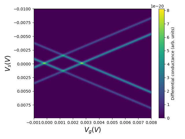
Fig. 2.4.5 Coulomb diamond
The "diamonds" manifest the so-called Coulomb blockade regions in which the source-to-drain and gate voltage configuration determines a quantized electron occupation number due to Coulomb repulsion. Because we only have 1 spin-degenerate state in our calculation, there is a maximal number of two electrons permitted in the dot. The first half diamond indicates the voltage configurations with no electrons, the full diamond with 1 electron and the final half diamond with 2 electrons.
In the next tutorial (NEGF–Poisson simulations of an FD-SOI field-effect transistor with a quantum dot), we will study transport through a single quantum dot using the Non-Equilibrium Green’s Function (NEGF) technique, which enables to relaxe many of the above assumptions required for validity of the WKB approximation, but treats Coulomb interactions between electrons in the channel in an approximate mean-field manner.
2.5. Full code
__copyright__ = "Copyright 2022-2026, Nanoacademic Technologies Inc."

import numpy as np
from matplotlib import pyplot as plt
import pathlib
from progress.bar import ChargingBar as Bar
from qtcad.device.mesh3d import Mesh, SubMesh
from qtcad.device import constants as ct
from qtcad.device import materials as mt
from qtcad.device import Device, SubDevice
from qtcad.device.schrodinger import Solver
from qtcad.device.schrodinger import SolverParams as SingleBodySolverParams
from qtcad.device.many_body import SolverParams as ManyBodySolverParams
from qtcad.transport.junction import Junction
from qtcad.transport.lead import WKBLead
from qtcad.transport.mastereq import seq_tunnel_curr

# Paths to mesh file and output files
script_dir = pathlib.Path(__file__).parent.resolve()
path_mesh = script_dir / "meshes/" / "lead_dot_lead.msh"
scalingFactor = 1e-9
mesh = Mesh(scalingFactor, str(path_mesh))

# Create the device from the mesh
d = Device(mesh, conf_carriers="e")

d.new_region("dot", mt.GaAs)
d.new_region("lead", mt.GaAs)
d.new_region("lead2", mt.GaAs)
d.new_region("barrier", mt.GaAs)
d.new_region("barrier2", mt.GaAs)

# Global nodes
x = mesh.glob_nodes[:, 0]
y = mesh.glob_nodes[:, 1]
z = mesh.glob_nodes[:, 2]

# Potential along y and z
# Position of the harmonic oscillator minimum
y0 = 0
z0 = 0
Ky = 2e-7  # Parabolic in y
Kz = 1e-4  # Parabolic in z
Vy = Ky / 2.0 * (y - y0) ** 2
Vz = Kz / 2.0 * (z - z0) ** 2
# Set the potential energy
d.set_V(Vy + Vz)

# Add the potential energy along x
d.add_to_V(12e-3 * ct.e, region="barrier")
d.add_to_V(12e-3 * ct.e, region="barrier2")
d.add_to_V(-10e-3 * ct.e, region="lead")
d.add_to_V(-10e-3 * ct.e, region="lead2")
d.add_to_V(-1e-2 * ct.e)

# Create submesh
dotmesh = SubMesh(d.mesh, ["dot", "barrier", "barrier2"])
# Create subdevice
dot = SubDevice(d, dotmesh)
# Solve the Schrodinger equation.
# Configure the Schrödinger solver
params_schrod = SingleBodySolverParams()
params_schrod.num_states = 10  # Number of energy levels to consider
params_schrod.tol = 1e-9  # Set the tolerance for convergence

# Create solver
s = Solver(dot, solver_params=params_schrod)
s.solve()  # solve

# Take linecuts to define lead potential
# Length of dot region
L_dot = 200 * scalingFactor
# Length of left lead
L_lead1 = 50 * scalingFactor
# Length of right lead
L_lead2 = 50 * scalingFactor

x0 = L_lead1 - 10 * scalingFactor
x0R = L_lead1 + L_dot + 10 * scalingFactor

L_intersection = (x0, y0, z0)
R_intersection = (x0R, y0, z0)

# Define the leads.
mass = 1 / mt.GaAs.Me_inv[0, 0]
R_lead = WKBLead(
    d,
    ["dot", "barrier", "barrier2"],
    R_intersection,
    "x",
    ["lead2"],
    mass=mass,
    n1=1,
    n2=1,
    extra_region=["lead"],
)
L_lead = WKBLead(
    d,
    ["dot", "barrier", "barrier2"],
    L_intersection,
    "x",
    ["lead"],
    mass=mass,
    n1=1,
    n2=1,
    extra_region=["lead2"],
)

# Plot lead wavefunctions for a given energy
Etest = 5e-3 * ct.e
R_lead.plot_lead_wf(Etest, 0, 0, "x", "y", "z")
L_lead.plot_lead_wf(Etest, 0, 0, "x", "y", "z")

# Define the junction (left lead - dot - right lead)
many_body_solver_params = ManyBodySolverParams()
many_body_solver_params.num_states = 1
many_body_solver_params.n_degen = 2
junc = Junction(dot, L_lead, R_lead, many_body_solver_params=many_body_solver_params)

junc.set_temperature(1)  # set temperature in unit of K
# Tunnelling computed using the WKB approximation
# Set source and drain voltages to low-bias regime
junc.setVs(2.5e-3)  # set source voltage in volts
junc.setVd(0.0)  # set drain voltage in volts

# Compute Coulomb peaks
v_gate_rng = np.linspace(-0.001, 0.008, num=100)
currentl = []

# Progress bar for the calculation of the Coulomb peaks
number_points = v_gate_rng.size  # number of sampled voltages
progress_bar_peaks = Bar("Computing Coulomb peaks", max=number_points)

for V in v_gate_rng:  # loop over gate voltage
    junc.setVg(V)
    Il, Ir, prob = seq_tunnel_curr(junc)  # transport calculation
    currentl.append(-Il)
    progress_bar_peaks.next()

progress_bar_peaks.finish()

I = np.array(currentl)

# Plot
fig, ax = plt.subplots(1)
ax.set_xlabel("Gate voltage (V)")
ax.set_ylabel("Current (nA)")
ax.plot(v_gate_rng, -I / 1e-9)

plt.show()

# For visualization purposes only: uniform rates assumed for all transitions.
junc.WKB = False  # 'Turn off' WKB approximation

# Compute Coulomb diamonds.
v_gate_rng = np.linspace(-0.001, 0.008, num=150)
v_left_rng = np.linspace(-0.01, 0.01, num=150)
diam = np.zeros((v_gate_rng.size, v_left_rng.size), dtype=float)

# Progress bar for the calculation of the Coulomb diamonds
number_grid_points = v_gate_rng.size * v_left_rng.size  # number of sampled grid points
progress_bar_diamond = Bar("Computing charge stability diagram", max=number_grid_points)

for i in range(v_gate_rng.size):  # loop over gate voltage
    v_gate = v_gate_rng[i]
    junc.setVg(v_gate)
    for j in range(v_left_rng.size):  # loop over source/drain voltage
        v_left = v_left_rng[j]
        junc.setVs(v_left)
        # drain voltage is assumed to be opposite to source
        junc.setVd(-v_left)
        Il, Ir, prob = seq_tunnel_curr(junc)  # transport calculation
        diam[i, j] = Il
        progress_bar_diamond.next()

progress_bar_diamond.finish()

diam = np.abs(diam[:, 1:] - diam[:, :-1])  # differential conductance

# plot results
fig, axs = plt.subplots()
axs.set_ylabel("$V_s(V)$", fontsize=16)
axs.set_xlabel("$V_g(V)$", fontsize=16)
diff_cond_map = axs.imshow(
    np.transpose(diam),
    interpolation="bilinear",
    extent=[v_gate_rng[0], v_gate_rng[-1], v_left_rng[-2], v_left_rng[0]],
    aspect="auto",
)
fig.colorbar(diff_cond_map, ax=axs, label="Differential conductance (arb. units)")
fig.tight_layout()
plt.show()