3. Quantum transport—Charge stability diagram of a double quantum dot
3.1. Requirements
3.1.1. Software components
QTCAD®
Gmsh
3.1.2. Geometry file
qtcad/examples/tutorials/meshes/dqdfdsoi.geo
3.1.3. Python script
qtcad/examples/tutorials/double_dot_stability.py
3.1.4. References
Generalization to multiple-dot systems: Lever arm matrix theory section.
A simplified many-body Hamiltonian: The Fermi–Hubbard model theory section.
Particle addition spectrum theory section.
A double quantum dot device in a fully-depleted silicon-on-insulator transistor tutorial.
3.2. Briefing
In this tutorial, we will use QTCAD to calculate the charge stability diagram of a double quantum dot in a generic fully-depleted silicon-on-insulator (FD-SOI) structure.
3.3. Computational approach
A charge stability diagram is typically obtained by measuring the current or the differential conductance of a double quantum dot system as a function of a pair of plunger gate potentials used to control the chemical potentials of each dot.
Several workflows could be applied for double dot charge stability diagram calculations. In the most complete calculation, for each gate bias configuration, one would successively solve the Poisson, Schrödinger, many-body, and master equations to compute the current flowing through the system. While this approach enables to model confinement potential variations with plunger gate biases, it is also computationally expensive.
In many situations, one is content with identifying the location of transition lines in the charge stability diagram. In such situations, it is possible to considerably accelerate the calculation with the following approximations:
Lever arm approximation: As described in Generalization to multiple-dot systems: Lever arm matrix, we may approximate the effect of plunger gate bias variations as linear changes in the double dot single-particle energy levels through a lever arm matrix, which is closely related to the capacitance matrix of the system. Through this approximation, one can avoid solving the Poisson, single-particle Schrödinger, and many-body Schrödinger equations again for each new bias configuration.
Hubbard model approximation: As described in A simplified many-body Hamiltonian: The Fermi–Hubbard model, by neglecting overlaps between single-particle eigenstates, the Coulomb interaction matrix may be computed considerably faster by reducing the number of integrals from \(\mathcal O(n_\mathrm{states}^4)\) to \(\mathcal O(n_\mathrm{states}^2)\).
Near-equilibrium response function: Instead of solving the master equation for the many-body system to compute the current, it is possible to use a simpler approach based on equilibrium statistical mechanics, as described in the Particle addition spectrum theory section, to calculate the particle addition spectrum. While this approach does not directly yield the current or differential conductance, it does enable to calculate the location of transitions in charge stability diagrams when the junction is nearly at equilibrium.
3.4. Device geometry
The device geometry considered here is explained and illustrated in the A double quantum dot device in a fully-depleted silicon-on-insulator transistor tutorial.
3.5. Geometry file
As before, the initial mesh is generated from a
geometry file qtcad/examples/tutorials/meshes/dqdfdsoi.geo
by running Gmsh with
gmsh dqdfdsoi.geo
As in Tunnel coupling in a double quantum dot in FD-SOI—Part 1: Plunger gate tuning, this will produce a .msh file and a
.xao file. The .xao file format is appropriate for
geometries produced using the OpenCASCADE geometry kernel.
3.6. Header
We start with importing the necessary packages
import numpy as np
import pathlib
from matplotlib import pyplot as plt
from progress.bar import ChargingBar as Bar

from qtcad.device import constants as ct
from qtcad.device import analysis as an
from qtcad.device.mesh3d import Mesh, SubMesh
from qtcad.device import SubDevice
from qtcad.device.poisson import Solver as PoissonSolver
from qtcad.device.poisson import SolverParams as PoissonSolverParams
from qtcad.device.schrodinger import Solver as SchrodingerSolver
from qtcad.device.schrodinger import SolverParams as SchrodingerSolverParams
from qtcad.device.many_body import Solver as ManyBodySolver
from qtcad.device.many_body import SolverParams as ManyBodySolverParams
from qtcad.device.leverarm_matrix import Solver as LeverArmSolver
from qtcad.device.leverarm_matrix import SolverParams as LeverArmSolverParams
from qtcad.transport.junction import Junction
from qtcad.transport.mastereq import add_spectrum
from helper.double_dot_fdsoi import get_double_dot_fdsoi
The following modules or functions were not covered in previous tutorials:
leverarm_matrix: A generalization of the lever arm module for multiple-dot systems.add_spectrum: A function of themastereqmodule that calculates the particle addition spectrum at equilibrium instead of solving the full master equation.
Finally, we import the get_double_dot_fdsoi function from the
A double quantum dot device in a fully-depleted silicon-on-insulator transistor tutorial to produce an appropriate
Device object for the FD-SOI structure.
3.7. Setting up the device
3.7.1. Importing the mesh
After producing the mesh with
gmsh examples/tutorials/meshes/dqdfdsoi.geo
we define paths and import the mesh with the usual methods.
# Set up paths
script_dir = pathlib.Path(__file__).parent.resolve()

# Mesh path
path_mesh = script_dir / "meshes"
path_out = script_dir / "output"

# Load the mesh
scaling = 1e-9
mesh = Mesh(scaling, str(path_mesh / "dqdfdsoi.msh"))
3.7.2. Defining the device
In this tutorial, a function generating a
Device object for a double quantum dot
in FD-SOI is defined. The function takes as arguments a 3D
Mesh object, along with biases for each
gate. We first define variables for the gate biases with:
# Define the gate bias parameters
back_gate_bias = -0.5
barrier_gate_1_bias = 0.5
plunger_gate_1_bias = 0.6
barrier_gate_2_bias = 0.5
plunger_gate_2_bias = 0.6+1e-3
barrier_gate_3_bias = 0.5
and then define the
Device object
# Define the device object from the function defined in the FD-SOI tutorial
dvc = get_double_dot_fdsoi(mesh, back_gate_bias, barrier_gate_1_bias,
   plunger_gate_1_bias, barrier_gate_2_bias, plunger_gate_2_bias,
   barrier_gate_3_bias)
We recall that for this device, confined carriers are electrons, and temperature is set to \(100~\mathrm{mK}\).
In addition, we have chosen a gate bias configuration that leads to a nearly symmetric double quantum dot configuration. We choose the two plunger gate biases to have a weak detuning (\(1~\mathrm{meV}\)) to ensure that the resulting single-electron eigenstates are localized within a single dot. The reason why this is necessary will be further explained in the Electrostatics in reference bias configuration section, below.
Finally, we define a list of region labels that, taken together, define the dot region in which classical charge densities are set to zero. This list will be used later when setting up non-linear Poisson and Schrödinger solvers.
# List of regions forming the double quantum dot region
dot_region_list = ["oxide_dot", "gate_oxide_dot", "buried_oxide_dot",
                  "channel_dot"]
3.8. Simulating the device
3.8.1. Configuring solvers
We then configure the parameters for the non-linear Poisson and single-electron Schrödinger solvers.
For the non-linear Poisson solver, we use adaptive meshing to facilitate convergence at cryogenic temperature. See the Poisson solver with adaptive meshing and Adaptive-mesh Poisson solver combined with the Schrödinger solver tutorials for a detailed explanation of non-linear Poisson solver parameters.
# Configure the non-linear Poisson solver
params_poisson = PoissonSolverParams()
params_poisson.tol = 1e-3 # Convergence threshold (tolerance) for the error
params_poisson.initial_ref_factor = 0.1
params_poisson.final_ref_factor = 0.75
params_poisson.min_nodes = 50000
params_poisson.max_nodes = 1e5
params_poisson.maxiter_adapt = 30
params_poisson.maxiter = 200
params_poisson.refined_region = dot_region_list
params_poisson.h_refined = 0.8
params_poisson.size_map_filename = str(path_mesh / "refined_dqdfdsoi.pos")
params_poisson.refined_mesh_filename = str(path_mesh / "refined_dqdfdsoi.msh")

# Number of single-electron orbital states to be considered
num_states = 4

# Instantiate Schrodinger solver's parameters
params_schrod = SchrodingerSolverParams()
params_schrod.num_states = num_states    # Number of states to consider
3.8.2. Electrostatics in reference bias configuration
Now that the material composition of the device and the external voltages have been specified, we successively solve the nonlinear Poisson equation in the entire device and Schrödinger’s equation in the dot region.
# Instantiate Poisson solver
poisson_slv = PoissonSolver(dvc, solver_params=params_poisson,
   geo_file=str(path_mesh/"dqdfdsoi.xao"))

# Solve Poisson's equation
poisson_slv.solve()

# Get the potential energy from the band edge for usage in the Schrodinger
# solver
dvc.set_V_from_phi()

# Create a submesh including only the dot region
submesh = SubMesh(dvc.mesh, dot_region_list)

# Create a subdevice for the dot region
subdvc = SubDevice(dvc, submesh)

# Create a Schrodinger solver
schrod_solver = SchrodingerSolver(subdvc, solver_params=params_schrod)

# Solve Schrodinger's equation
schrod_solver.solve()

# Output and save single-particle energy levels
subdvc.print_energies()
energies = subdvc.energies
np.save(path_out/"dqdfdsoi_energies.npy",energies)

# Plot single-electron eigenstates
x_slice = 0;  z_slice=-2e-9
an.plot_slices(subdvc.mesh,subdvc.eigenfunctions[:,0],
   title="Ground state", x=x_slice, z=z_slice)
an.plot_slices(subdvc.mesh,subdvc.eigenfunctions[:,1],
   title="First excited state", x=x_slice, z=z_slice)
an.plot_slices(subdvc.mesh,subdvc.eigenfunctions[:,2],
   title="Second excited state", x=x_slice, z=z_slice)
an.plot_slices(subdvc.mesh,subdvc.eigenfunctions[:,3],
   title="Third excited state", x=x_slice, z=z_slice)
The above code snippet prints the single-electron orbital energy levels:
Energy levels (eV)
[0.04112597 0.04183574 0.04604206 0.04680443]
In addition, the corresponding wave functions are plotted as follows.
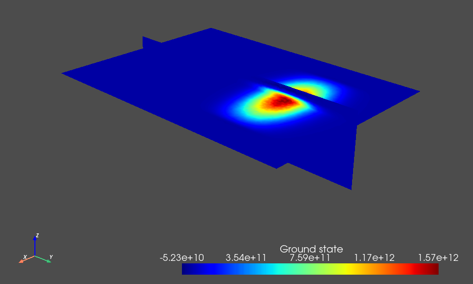
Fig. 3.8.1 Single-electron ground state.
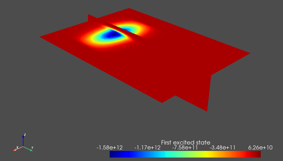
Fig. 3.8.2 Single-electron first excited state.
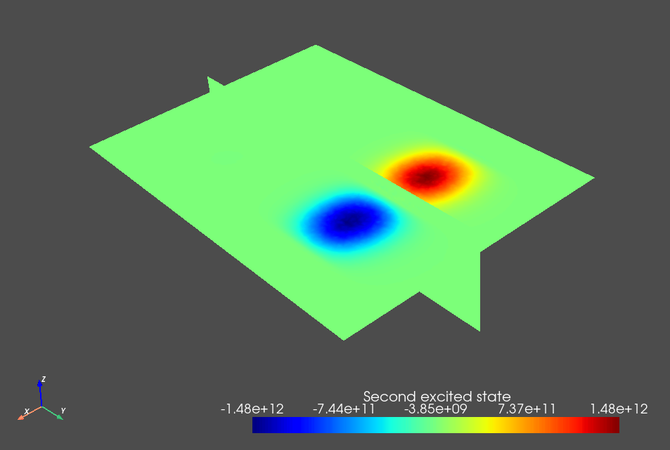
Fig. 3.8.3 Single-electron second excited state.
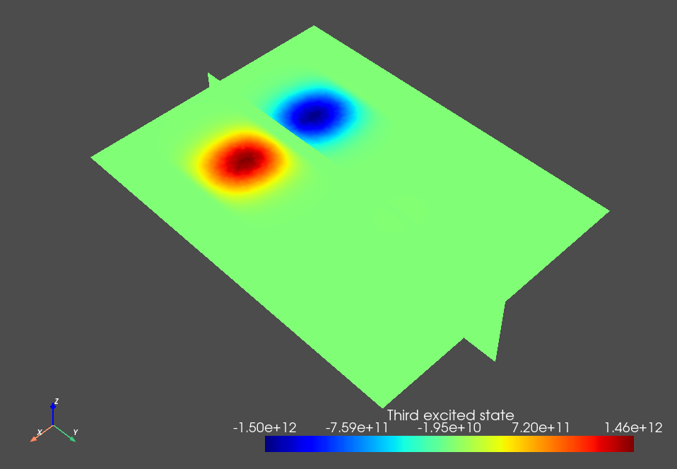
Fig. 3.8.4 Single-electron third excited state.
The weak detuning between the plunger gates leads to a detuning of the double dot potential minima that dominates over its tunnel splitting and thus ensures that the orbital states are localized in each dot. This is key to the simplified charge stability diagram workflow presented below because we will assume a localized basis set when calculating the lever arm and Coulomb interaction matrices.
3.9. Lever arm matrix calculation
Biasing a gate generally has a finite impact over the entire confinement potential profile. In the most general calculation, the Poisson and Schrödinger equations are solved again in each bias configuration.
However, when computing charge stability diagrams, solving these two equations for each new bias configuration is very time consuming because several hundreds of bias configurations may have to be explored.
Therefore, we consider the lever arm matrix approximation presented in Generalization to multiple-dot systems: Lever arm matrix, in which single-electron energy levels are approximated by Eq. (6.6).
To calculate the lever arm matrix, we instantiate a lever arm matrix
Solver object from the
leverarm_matrix module.
The constructor of the
Solver
class takes as mandatory inputs a device, a list of labels corresponding
to gate boundaries for which the effect of gate biases are considered,
and a bias vector containing the applied potential at each such gate boundary
in the reference configuration. In addition, a list specifying the dot region
and a lever arm matrix
SolverParams object are
provided as optional arguments.
The lever_arm_matrix
SolverParams, lam_params,
contains Poisson SolverParams
and Schrödinger SolverParams
used internally by the Solver to
compute the lever arm matrix.
# Instantiate the voltage bias vector
bias_vector = np.array([plunger_gate_1_bias, plunger_gate_2_bias])

# Bias labels
gate_labels = ["plunger_gate_1_bnd", "plunger_gate_2_bnd"]

# Solver params for the LeverArmSolver
lam_params = LeverArmSolverParams()
lam_params.pot_solver_params = params_poisson
lam_params.schrod_solver_params = params_schrod

# Instantiate lever arm matrix solver
slv = LeverArmSolver(dvc, gate_labels, bias_vector, dot_region=dot_region_list,
   solver_params=lam_params)
Upon calling the
solve method, the
Poisson and Schrödinger equations are successively solved in several gate bias
configurations to evaluate the lever arm matrix. The first configuration
to be considered is the reference configuration defined by the bias_vector.
After solving the Poisson and Schrödinger equations in this configuration,
the same equations are solved in all possible configurations that differ from
reference by a bias increment on one of the gates, enabling
evaluation of the lever arm matrix from first-order finite differences.
This procedure is followed below with a finite-difference increment of \(1~\mathrm{mV}\).
# Calculate the lever arm matrix
bias_increment = 1e-3
lever_arm_matrix = slv.solve(bias_increment=bias_increment)

# Print and save the lever arm matrix
print("Lever arm matrix")
print(lever_arm_matrix)
np.save(path_out/"lever_arm_matrix.npy", lever_arm_matrix)
After a few minutes, the calculation is finished, and the lever arm matrix is output as:
[[0.00621886 0.76474834]
[0.76471827 0.00618066]
[0.00595462 0.7646695 ]
[0.76424525 0.00622768]]
Here, dot 2 is biased with a slightly larger plunger gate bias than dot 1, causing the ground state of dot 2 to be below that of dot 1. Since energy levels are sorted from the lowest to the highest when solving Schrödinger’s equation, the rows in the above matrix correspond to the ground state of dot 2, the ground state of dot 1, the first excited state of dot 2, and the first excited state of dot 1, respectively. In addition, the columns correspond to plunger gate 1 and plunger gate 2. We conclude that the cross-capacitance between the plunger gates of opposite dots is very small in this example (\(\approx 0.006\)), most likely because the gate oxide layer is very thin compared with the distance between the dots.
3.10. Coulomb interaction matrix calculation
For weak overlap between single-body states, we model interactions between electrons using the Fermi–Hubbard model defined by Eq. (8.15). For a basis set containing \(n_\mathrm{states}\) single-particle orbitals, the number of Coulomb integrals to evaluate then scales like \(\mathcal O(n_\mathrm{states}^2)\) instead of the more expensive \(\mathcal O (n_\mathrm{states}^4)\) scaling achieved when including overlap terms.
To compute the Coulomb interaction terms \(U_i\) and
\(V_{ij}\) appearing in the model, we use the method
get_coulomb_matrix
of the many-body
Solver
class, making sure to set the optional argument overlap to False.
This is done in the code block that follows.
# Calculate the Coulomb interaction matrix
# Instantiate many-body solver
many_body_solver_params = ManyBodySolverParams()
many_body_solver_params.n_degen = 2
many_body_solver_params.num_states = num_states
slv = ManyBodySolver(subdvc, solver_params=many_body_solver_params)

# Compute, save, and print Coulomb interaction matrix without overlap terms
coulomb_no_overlap = slv.get_coulomb_matrix(overlap=False, verbose=True)
np.save(path_out/"coulomb_mat_no_overlap.npy", coulomb_no_overlap)
print("Coulomb interaction matrix (eV)")
print(coulomb_no_overlap/ct.e)

# Compute and save Coulomb interaction matrix with overlap terms
# coulomb_overlap = slv.get_coulomb_matrix(verbose=True, overlap=True)
# np.save(path_out/"full_coulomb_mat.npy", coulomb_overlap)
When printing the Coulomb interaction matrix without overlap, we obtain
[[0.01843589 0.00330611 0.01466883 0.00323352]
[0.00330611 0.01849507 0.00323617 0.01467277]
[0.01466883 0.00323617 0.01544532 0.00317834]
[0.00323352 0.01467277 0.00317834 0.01545166]]
The above array corresponds to \(V_{ij} = V_{ijij}\), so that the diagonal elements of the array give interactions \(U_i=V_{iiii}\) between electrons occupying the same single-electron orbital, while off-diagonal elements give interactions between electrons occupying distinct orbitals. Since rows and columns are ordered from the lowest-energy to the highest-energy single-electron state, as can be seen from Fig. 3.8.1 to Fig. 3.8.4, rows 0 (1) and 2 (3) correspond to orbitals localized in dot 2 (1). Therefore, as could be expected intuitively, interactions between electrons occupying the same dot are much stronger than interactions between electrons in different dots. Remark that since the double dot configuration is nearly symmetric, and Gmsh may produce slightly different outputs betwen workstations and operating systems, it is possible that the specific order of eigenstates be different on your platform, leading to permutations in the above Coulomb interaction matrix. This should however not significantly affect the charge stability diagram simulated below.
Finally, the commented part of the above code block enables to calculate the full 4D Coulomb interaction matrix \(V_{ijkl}\) including overlap terms. Since this calculation is more time consuming, we do not perform it here. However, in certain circumstances, the overlap term may have a significant impact on the charge stability diagram. In such cases, a larger computational expense is paid upfront by calculating the Coulomb interaction matrix. However, within the lever arm approximation, this step only needs to be completed once, and the charge stability diagram itself may still be calculated efficiently using the method described here.
3.11. Charge stability diagram calculation
After computing the single-particle and many-body electronic structure of our double quantum dot system, it is now time to consider its charge stability diagram.
In the most complete workflow currently achievable with QTCAD, the current
flowing through the structure is calculated by solving a
master equation
with tunneling rates computed from the
WKB approximation.
This can easily be done by instantiating a
Junction object with WKB
leads, and using the
seq_tunnel_curr
of the
mastereq module.
However, in many cases, this approach can be time consuming. When simply
attempting to determine which bias configurations lead to the single-electron
regime (i.e., locating transition lines in a charge stability diagram), it
may be more appropriate to speed up calculations by introducing an additional
approximation.
When the source–drain bias is sufficiently weak, the double quantum dot system is nearly at thermodynamic equilibrium with the leads. The location of the transition lines in the charge stability diagram may then be identified by calculating the average particle addition spectrum in the grand canonical ensemble, which is given by Eq. (10.15) of the Particle addition spectrum theory section. Because the Fermi–Hubbard Hamiltonian is already diagonal in the particle-number basis, calculating the particle addition spectrum for a small number of electrons is a computationally cheap task.
To compute the charge stability diagram with the particle addition spectrum
method, we will use the
add_spectrum function of the
mastereq module, which takes as input a
Junction object that was
previously instantiated using appropriate parameters of the multiple dot
system. We instantiate this junction with:
# Set the junction temperature to 10 K (instead of 100 mK) to make lines
# in the charge stability diagram thicker and decrease the resolution
# required to observe them
temperature_spec = 10

# Contact labels
gate_labels = ["source_bnd", "plunger_gate_1_bnd", "plunger_gate_2_bnd",
   "drain_bnd"]

# Instantiate a junction
many_body_solver_params.energies = energies
many_body_solver_params.overlap = False
many_body_solver_params.coulomb_mat = coulomb_no_overlap
many_body_solver_params.alpha = lever_arm_matrix
jc = Junction(many_body_solver_params = many_body_solver_params,
   temperature=temperature_spec, contact_labels=gate_labels)
In contrast with the approaches presented in the
master equation and
WKB approximation tutorials, here, we do not instantiate
the Junction from a
Device or
SubDevice object.
Instead, to instantiate the junction, we use a many-body
SolverParams
object that contains the single-particle energy levels, the Coulomb interaction
matrix, and the lever arm matrix arrays that were previously calculated.
This will have two effects:
Avoiding to recalculate Coulomb integrals upon
Junctioninstantiation.Introducing the lever arm matrix approximation, according to which single-body energies in the Hamiltonian may be recalculated when modifying gate biases without having to solve the single-particle Schrödinger equation again.
Additional optional arguments and solver parameters specified above are:
temperature: the junction temperature used when solving the master equation or computing the particle addition spectrum. Here, we set this temperature to \(10~\mathrm{K}`\) instead of the \(100~\mathrm{mK}\) value taken in electrostatics calculation to broaden transition lines and decrease the resolution required in the charge stability diagram to observe them. Lower temperatures may be considered at the cost of increased computation time.overlap: whether or not the Coulomb interaction matrix includes overlap terms.gate_labels: the string labels of the contacts at the source and drain, and of the gates used to manipulate the dot energy levels (typically plunger gates). By convention, the first and last labels in this list must be those of the source and drain.
After instantiating the Junction, we define a function that will be used to set its gate bias configuration and compute the corresponding particle addition spectrum.
def get_add_spectrum(junc, gate_labels, gate_biases, temperature,
   verbose=True):
   """ Computes the response function of a double quantum dot for a given
   set of gate biases.

   Args:
      junc (transport junction object) : Junction object to consider.
      gate_labels (list): Labels of the gates at which biases are applied.
      gate_biases (ndarray) : Applied bias on each gate.
      temperature (float): Temperature to use in the particle addition
         spectrum.
      verbose (bool, optional): Verbosity level.

   Returns:
      float: The addition spectrum at the chosen gate bias configuration.
   """
   # Set list of biases with drain potential + increment
   junc.set_biases(gate_labels,gate_biases, verbose=verbose)

   # Calculate response function
   out = add_spectrum(junc, temperature=temperature)
   return out
Setting both source and drain potentials to zero, we then loop over plunger gate biases, calculate the particle addition spectrum for each plunger gate bias configuration, and store it in an array.
# Base source and drain potentials
source_potential = 0
drain_potential = 0

# Extremal values of the gate biases
min_gate_1_bias = 30e-3 ; max_gate_1_bias = 140e-3
min_gate_2_bias = 30e-3 ; max_gate_2_bias = 140e-3

gate_1_biases = np.linspace( min_gate_1_bias, max_gate_1_bias, 90)
gate_2_biases = np.linspace( min_gate_2_bias, max_gate_2_bias, 90)
add_spectrum_mat = np.zeros((len(gate_1_biases),len(gate_2_biases)))

bartitle = "Calculating charge stability diagram."
progress_bar = Bar(bartitle, max = len(gate_1_biases)*len(gate_1_biases))
for idx_1, gate_1_bias in enumerate(gate_1_biases):
   for idx_2, gate_2_bias in enumerate(gate_2_biases):
      add_spectrum_mat[idx_1,idx_2] =\
            get_add_spectrum(jc, gate_labels, np.array([source_potential,
               gate_1_bias, gate_2_bias, drain_potential]), temperature_spec,
               verbose=False)
      np.savetxt(path_out / "addition_spectrum.txt", add_spectrum_mat)
      progress_bar.next()

progress_bar.finish()
Note
Here, the gate biases are expressed with respect to the reference
configuration in which device electrostatics were first calculated.
For example, if, in the above loop, gate_1_bias = 100 mV, the potential
that is actually applied on plunger gate 1 is
plunger_gate_1_bias + gate_1_bias = 0.601 V.
3.12. Plotting the results
We finally plot the results stored in the add_spectrum_mat array using
PyPlot.
# Plot the particle addition spectrum
# Transpose and flip the matrix to turn into an image with bias_1 along x
# and bias_2 along y
add_spec_to_plot = np.flip(np.transpose(add_spectrum_mat),axis=0)
fig, axs = plt.subplots()
axs.set_xlabel('$V_{g1}$ (V)',fontsize=16)
axs.set_ylabel('$V_{g2}$ (V)',fontsize=16)
vg1_ref = plunger_gate_1_bias; vg2_ref = plunger_gate_2_bias;
diff_conds_map = axs.imshow(add_spec_to_plot/np.max(add_spec_to_plot),
      cmap="jet", interpolation='bilinear',
      extent=[min_gate_1_bias+vg1_ref, max_gate_1_bias+vg1_ref,
            min_gate_2_bias+vg2_ref, max_gate_2_bias+vg2_ref], aspect="auto")
fig.colorbar(diff_conds_map, ax=axs, label="Response (arb. units)")
fig.tight_layout()
plt.show()
This results in the following charge stability diagram.
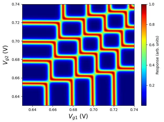
Fig. 3.12.1 Particle addition spectrum as a function of plunger gate biases in the FD-SOI structure presented here.
The transition lines are associated with changes in the total particle numbers. These lines enable to distinguish distinct charge configurations in the double quantum dot. Labeling charge states with the notation \((m_1,m_2)\), where \(m_1\) (\(m_2\)) is the total number of electrons in dot 1 (2), we obtain the diagram shown below.
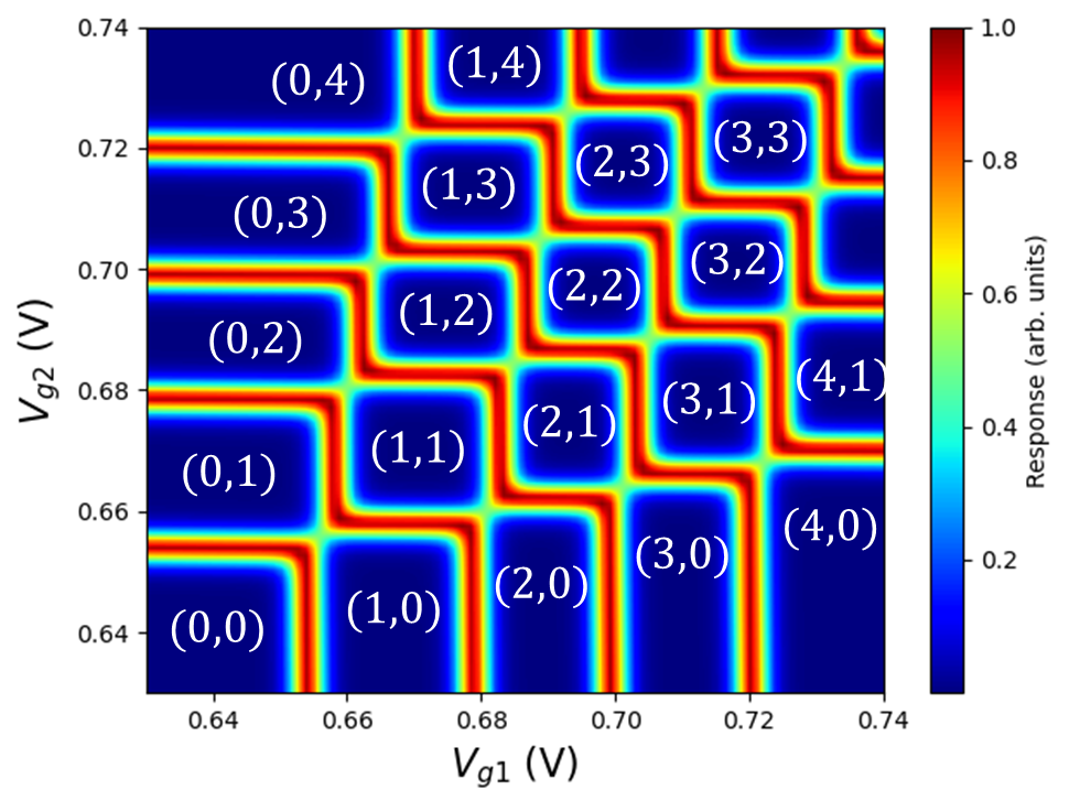
Fig. 3.12.2 Charge stability diagram with labeled dot occupations.
In addition, the slopes of the transition lines are determined by the lever arm matrix. Nearly orthogal lines such as those seen here indicate a lever arm matrix that does not significantly couple the plunger gates of a dot to the other (i.e., cross-capacitance effects are negligible). As alluded to above, in the structure studied here, this can be attributed to thinness of the gate oxide layer compared with the distance between the dots. For thicker gate oxides, transition lines would intersect at more obtuse angles.
3.13. Full code
__copyright__ = "Copyright 2022-2026, Nanoacademic Technologies Inc."

import numpy as np
import pathlib
from matplotlib import pyplot as plt
from progress.bar import ChargingBar as Bar
from qtcad.device import constants as ct
from qtcad.device import analysis as an
from qtcad.device.mesh3d import Mesh, SubMesh
from qtcad.device import SubDevice
from qtcad.device.poisson import Solver as PoissonSolver
from qtcad.device.poisson import SolverParams as PoissonSolverParams
from qtcad.device.schrodinger import Solver as SchrodingerSolver
from qtcad.device.schrodinger import SolverParams as SchrodingerSolverParams
from qtcad.device.many_body import Solver as ManyBodySolver
from qtcad.device.many_body import SolverParams as ManyBodySolverParams
from qtcad.device.leverarm_matrix import Solver as LeverArmSolver
from qtcad.device.leverarm_matrix import SolverParams as LeverArmSolverParams
from qtcad.transport.junction import Junction
from qtcad.transport.mastereq import add_spectrum
from helper.double_dot_fdsoi import get_double_dot_fdsoi

# Set up paths
script_dir = pathlib.Path(__file__).parent.resolve()

# Mesh path
path_mesh = script_dir / "meshes"
path_out = script_dir / "output"

# Load the mesh
scaling = 1e-9
mesh = Mesh(scaling, str(path_mesh / "dqdfdsoi.msh"))

# Define the gate bias parameters
back_gate_bias = -0.5
barrier_gate_1_bias = 0.5
plunger_gate_1_bias = 0.6
barrier_gate_2_bias = 0.5
plunger_gate_2_bias = 0.6 + 1e-3
barrier_gate_3_bias = 0.5

# Define the device object from the function defined in the FD-SOI tutorial
dvc = get_double_dot_fdsoi(
    mesh,
    back_gate_bias,
    barrier_gate_1_bias,
    plunger_gate_1_bias,
    barrier_gate_2_bias,
    plunger_gate_2_bias,
    barrier_gate_3_bias,
)

# List of regions forming the double quantum dot region
dot_region_list = ["oxide_dot", "gate_oxide_dot", "buried_oxide_dot", "channel_dot"]

# Configure the non-linear Poisson solver
params_poisson = PoissonSolverParams()
params_poisson.tol = 1e-3  # Convergence threshold (tolerance) for the error
params_poisson.initial_ref_factor = 0.1
params_poisson.final_ref_factor = 0.75
params_poisson.min_nodes = 50000
params_poisson.max_nodes = 1e5
params_poisson.maxiter_adapt = 30
params_poisson.maxiter = 200
params_poisson.refined_region = dot_region_list
params_poisson.h_refined = 0.8
params_poisson.size_map_filename = str(path_mesh / "refined_dqdfdsoi.pos")
params_poisson.refined_mesh_filename = str(path_mesh / "refined_dqdfdsoi.msh")

# Number of single-electron orbital states to be considered
num_states = 4

# Instantiate Schrodinger solver's parameters
params_schrod = SchrodingerSolverParams()
params_schrod.num_states = num_states  # Number of states to consider

# Instantiate Poisson solver
poisson_slv = PoissonSolver(
    dvc, solver_params=params_poisson, geo_file=str(path_mesh / "dqdfdsoi.xao")
)

# Solve Poisson's equation
poisson_slv.solve()

# Get the potential energy from the band edge for usage in the Schrodinger
# solver
dvc.set_V_from_phi()

# Create a submesh including only the dot region
submesh = SubMesh(dvc.mesh, dot_region_list)

# Create a subdevice for the dot region
subdvc = SubDevice(dvc, submesh)

# Create a Schrodinger solver
schrod_solver = SchrodingerSolver(subdvc, solver_params=params_schrod)

# Solve Schrodinger's equation
schrod_solver.solve()

# Output and save single-particle energy levels
subdvc.print_energies()
energies = subdvc.energies
np.save(path_out / "dqdfdsoi_energies.npy", energies)

# Plot single-electron eigenstates
x_slice = 0
z_slice = -2e-9
an.plot_slices(
    subdvc.mesh, subdvc.eigenfunctions[:, 0], title="Ground state", x=x_slice, z=z_slice
)
an.plot_slices(
    subdvc.mesh,
    subdvc.eigenfunctions[:, 1],
    title="First excited state",
    x=x_slice,
    z=z_slice,
)
an.plot_slices(
    subdvc.mesh,
    subdvc.eigenfunctions[:, 2],
    title="Second excited state",
    x=x_slice,
    z=z_slice,
)
an.plot_slices(
    subdvc.mesh,
    subdvc.eigenfunctions[:, 3],
    title="Third excited state",
    x=x_slice,
    z=z_slice,
)

# Instantiate the voltage bias vector
bias_vector = np.array([plunger_gate_1_bias, plunger_gate_2_bias])

# Bias labels
gate_labels = ["plunger_gate_1_bnd", "plunger_gate_2_bnd"]

# Solver params for the LeverArmSolver
lam_params = LeverArmSolverParams()
lam_params.pot_solver_params = params_poisson
lam_params.schrod_solver_params = params_schrod

# Instantiate lever arm matrix solver
slv = LeverArmSolver(
    dvc, gate_labels, bias_vector, dot_region=dot_region_list, solver_params=lam_params
)

# Calculate the lever arm matrix
bias_increment = 1e-3
lever_arm_matrix = slv.solve(bias_increment=bias_increment)

# Print and save the lever arm matrix
print("Lever arm matrix")
print(lever_arm_matrix)
np.save(path_out / "lever_arm_matrix.npy", lever_arm_matrix)

# Calculate the Coulomb interaction matrix
# Instantiate many-body solver
many_body_solver_params = ManyBodySolverParams()
many_body_solver_params.n_degen = 2
many_body_solver_params.num_states = num_states
slv = ManyBodySolver(subdvc, solver_params=many_body_solver_params)

# Compute, save, and print Coulomb interaction matrix without overlap terms
coulomb_no_overlap = slv.get_coulomb_matrix(overlap=False, verbose=True)
np.save(path_out / "coulomb_mat_no_overlap.npy", coulomb_no_overlap)
print("Coulomb interaction matrix (eV)")
print(coulomb_no_overlap / ct.e)

# Compute and save Coulomb interaction matrix with overlap terms
# coulomb_overlap = slv.get_coulomb_matrix(verbose=True, overlap=True)
# np.save(path_out/"full_coulomb_mat.npy", coulomb_overlap)

# Set the junction temperature to 10 K (instead of 100 mK) to make lines
# in the charge stability diagram thicker and decrease the resolution
# required to observe them
temperature_spec = 10

# Contact labels
gate_labels = ["source_bnd", "plunger_gate_1_bnd", "plunger_gate_2_bnd", "drain_bnd"]

# Instantiate a junction
many_body_solver_params.energies = energies
many_body_solver_params.overlap = False
many_body_solver_params.coulomb_mat = coulomb_no_overlap
many_body_solver_params.alpha = lever_arm_matrix
jc = Junction(
    many_body_solver_params=many_body_solver_params,
    temperature=temperature_spec,
    contact_labels=gate_labels,
)


def get_add_spectrum(junc, gate_labels, gate_biases, temperature, verbose=True):
    """Computes the response function of a double quantum dot for a given
    set of gate biases.

    Args:
       junc (transport junction object) : Junction object to consider.
       gate_labels (list): Labels of the gates at which biases are applied.
       gate_biases (ndarray) : Applied bias on each gate.
       temperature (float): Temperature to use in the particle addition
          spectrum.
       verbose (bool, optional): Verbosity level.

    Returns:
       float: The addition spectrum at the chosen gate bias configuration.
    """
    # Set list of biases with drain potential + increment
    junc.set_biases(gate_labels, gate_biases, verbose=verbose)

    # Calculate response function
    out = add_spectrum(junc, temperature=temperature)
    return out


# Base source and drain potentials
source_potential = 0
drain_potential = 0

# Extremal values of the gate biases
min_gate_1_bias = 30e-3
max_gate_1_bias = 140e-3
min_gate_2_bias = 30e-3
max_gate_2_bias = 140e-3

gate_1_biases = np.linspace(min_gate_1_bias, max_gate_1_bias, 90)
gate_2_biases = np.linspace(min_gate_2_bias, max_gate_2_bias, 90)
add_spectrum_mat = np.zeros((len(gate_1_biases), len(gate_2_biases)))

bartitle = "Calculating charge stability diagram."
progress_bar = Bar(bartitle, max=len(gate_1_biases) * len(gate_1_biases))
for idx_1, gate_1_bias in enumerate(gate_1_biases):
    for idx_2, gate_2_bias in enumerate(gate_2_biases):
        add_spectrum_mat[idx_1, idx_2] = get_add_spectrum(
            jc,
            gate_labels,
            np.array([source_potential, gate_1_bias, gate_2_bias, drain_potential]),
            temperature_spec,
            verbose=False,
        )
        np.savetxt(path_out / "addition_spectrum.txt", add_spectrum_mat)
        progress_bar.next()

progress_bar.finish()

# Plot the particle addition spectrum
# Transpose and flip the matrix to turn into an image with bias_1 along x
# and bias_2 along y
add_spec_to_plot = np.flip(np.transpose(add_spectrum_mat), axis=0)
fig, axs = plt.subplots()
axs.set_xlabel("$V_{g1}$ (V)", fontsize=16)
axs.set_ylabel("$V_{g2}$ (V)", fontsize=16)
vg1_ref = plunger_gate_1_bias
vg2_ref = plunger_gate_2_bias
diff_conds_map = axs.imshow(
    add_spec_to_plot / np.max(add_spec_to_plot),
    cmap="jet",
    interpolation="bilinear",
    extent=[
        min_gate_1_bias + vg1_ref,
        max_gate_1_bias + vg1_ref,
        min_gate_2_bias + vg2_ref,
        max_gate_2_bias + vg2_ref,
    ],
    aspect="auto",
)
fig.colorbar(diff_conds_map, ax=axs, label="Response (arb. units)")
fig.tight_layout()
plt.show()