6. Calculating the charge-stability diagram of a quantum dot

6.1. Requirements

6.1.1. Software components

• QTCAD

6.1.2. Mesh file

• qtcad/examples/practical_application/meshes/gated_dot.msh2

6.1.3. Python script

• qtcad/examples/practical_application/6-stability.py

6.1.4. References

• Calculating the Coulomb peaks of a quantum dot

• Transport in the Coulomb blockade regime

6.2. Briefing

In the previous tutorial, we computed the chemical potentials and Coulomb peaks of a quantum dot, two physical quantities important to describe transport in the dot. These computations explicitly assumed a fixed value of the plunger gates potential of \(-0.4\textrm{ V}\) and implicitly assumed a fixed value of the source–drain voltage of \(0\textrm{ V}\) (more specifically in the calculation of the Coulomb peak positions). In this tutorial, we expand on the ideas of the previous tutorial and describe transport in the quantum dot—specifically in terms of differential conductance—as a function of the plunger gates potential and of the source–drain voltage. We will eventually obtain the charge-stability diagram of our quantum dot, which can be used to infer the number of electrons in the dot; for example, which configurations of the external voltages result in a single electron residing in the dot?

6.3. Setting up the device

6.3.1. Header

We start by importing relevant modules.

import numpy as np
import pathlib
from matplotlib import pyplot as plt
import pickle
from progress.bar import ChargingBar as Bar

from device import constants as ct
from device.mesh3d import Mesh, SubMesh
from device import io

from device import Device, SubDevice
from device.schrodinger import Solver
from device.many_body import SolverParams
from transport.mastereq import seq_tunnel_curr
from transport.junction import Junction
from device import materials as mt

You will recognize most of these modules from previous tutorials with the exceptions of ChargingBar, seq_tunnel_curr, and junction. The ChargingBar module is used to print a progress bar during the calculation of the charge-stability diagram, which can take a few minutes or more. The seq_tunnel_curr method is used to compute the nonequilibrium statistics of a quantum dot and charge current due to sequential tunneling. Finally, the junction module is used to describe transport in a quantum dot coupled to two leads (source and drain) linearly.

6.3.2. Creating the junction

We start by defining the device as was previously done.

# Load the mesh
script_dir = pathlib.Path(__file__).parent.resolve()
path_mesh = str(script_dir/'meshes'/'gated_dot.msh2')
scaling = 1e-6
mesh = Mesh(scaling, path_mesh)

# Create device
d = Device(mesh, conf_carriers="e")
d.set_temperature(0.1)

# # Applied potentials
Vtop_1 = -0.5
Vtop_2 = -0.4
Vtop_3 = -0.5
Vbottom_1 = -0.5
Vbottom_2 = -0.4
Vbottom_3 = -0.5

# Work function of the metallic gates at midgap of GaAs
barrier = 0.834*ct.e    # n-type Schottky barrier height

# Ionized dopant density
doping = 3e18*1e6   # In SI units

# Set up materials in heterostructure stack
d.new_region("cap", mt.GaAs)
d.new_region("barrier", mt.AlGaAs)
d.new_region("dopant_layer", mt.AlGaAs,ndoping=doping)
d.new_region("spacer_layer", mt.AlGaAs)
d.new_region("spacer_dot", mt.AlGaAs)
d.new_region("two_deg", mt.GaAs)
d.new_region("two_deg_dot", mt.GaAs)
d.new_region("substrate", mt.GaAs)
d.new_region("substrate_dot", mt.GaAs)

# Remove unphysical charge from cap and barrier
d.new_insulator("cap")
d.new_insulator("barrier")

# Align the bands across hetero-interfaces using GaAs as the reference material
d.align_bands(mt.GaAs)

# Set up boundary conditions
d.new_schottky_bnd("top_gate_1", Vtop_1, barrier)
d.new_schottky_bnd("top_gate_2", Vtop_2, barrier)
d.new_schottky_bnd("top_gate_3", Vtop_3, barrier)
d.new_schottky_bnd("bottom_gate_1", Vbottom_1, barrier)
d.new_schottky_bnd("bottom_gate_2", Vbottom_2, barrier)
d.new_schottky_bnd("bottom_gate_3", Vbottom_3, barrier)
d.new_ohmic_bnd("ohmic_bnd")

# Load the confinement potential from previous run
path_in = str(script_dir/"output"/"electric_potential_-0.400V.hdf5")
d.set_potential(io.load(path_in))

# Create a submesh in which to solve Schrodinger's equation
submesh = SubMesh(mesh, ["spacer_dot","two_deg_dot","substrate_dot"])

# Create subdevice
subdevice = SubDevice(d, submesh)

# Solver the single-electron problem to get basis set
slv = Solver(subdevice)
slv.solve()
subdevice.print_energies()

We are now ready to define a junction, i.e. a quantum dot coupled to two leads (which we may call “source” and “drain”). Note that the coupling between the dot and the leads is linear, and may in the simplest approximation be described by a single parameter: a tunneling amplitude between the dot and the lead. In this simplest case, the leads need not be explicitly defined in the mesh or device object—even though they could be using the WKBLead class in more realistic simulations that explicitly account for the lead wave functions (see the Broadening function: WKB calculation theory section and the Quantum transport—WKB approximation tutorial).

many_body_solver_params = SolverParams()
many_body_solver_params.num_states = 2  # Number of levels to keep
many_body_solver_params.n_degen = 2     # spin degenerate system
many_body_solver_params.alpha = 0.0714  # lever arm
jc = Junction(subdevice, many_body_solver_params=many_body_solver_params)

print('chemical potentials (eV):', jc.chem_potentials/ct.e)
print('positions of Coulomb peaks relative to reference value (V):',
    jc.coulomb_peak_pos)

Upon instantiation, the Junction object creates and runs a many-body Solver to calculate the chemical potentials, Coulomb peak positions, and many-body eigenstates of the subdevice, which here corresponds to the quantum dot. Indeed, these quantities are all needed for transport calculations with the master-equation solver. Therefore, the arguments of the junction used above are the same as those of the many-body solver in Calculating the Coulomb peaks of a quantum dot, with the exception that the parameter num_states is set to 2 rather than 3 to speed up example calculations (num_states may easily be increased for improved accuracy at the expense of extended computation time).

After the Coulomb integrals calculation ends, the values of the chemical potentials and Coulomb peaks are printed.

chemical potentials (eV): [-0.00461879  0.00383573  0.01785463  0.02442585]
positions of Coulomb peaks relative to reference value (V): [-0.06468898  0.05372171  0.2500649   0.34209876]

Note

The position of the Coulomb peaks is given relative to the reference gate potential. The reference gate potential is the potential applied at the boundary condition when solving Poisson’s equation. Here, this reference potential is Vtop_2 = Vbottom_2 = -0.4 V, so that this value should be added to the above peak positions to find the true potentials to be applied at the gates to observe transport.

6.4. Computing the current as a function of plunger gates potential

As a first example for the seq_tunnel_curr method, we compute the sequential tunneling charge current of our quantum dot at fixed drain-to-source voltage and varying plunger gates potential. To do so, we first set the source and drain potentials using the setVs and setVd methods of the Junction class.

# Set a near-zero source-drain bias
jc.setVs(0.0001)
jc.setVd(-0.0001)

Next, we set a constant value of \(10\;\textrm{MHz}\) for the source and drain broadening functions within the featureless approximation (see The sequential tunneling master equation).

jc.set_source_broad_func(10e6)
jc.set_drain_broad_func(10e6)

Here, our drain-to-source voltage is \(0.2\textrm{ mV}\). The plunger gates potential is uniformly sampled from \(-0.1\textrm{ V}\) to \(0.4\textrm{ V}\).

v_gate_rng = np.linspace(-0.1, 0.4, num=200)

Next, we initialize an empty list vec_Il in which the sequential tunneling charge current as a function of gate potential will be stored. We then loop over the elements of v_gate_rng. In each iteration, the junction plunger gate potential is adjusted using the setVg method. We then call the seq_tunnel_curr method on the Junction object jc, which returns the current in the left lead (i.e. the source), Il, the current in the right lead (i.e. the drain), Ir, and the occupation rate of each quantum dot state, prob, as computed using a master-equation approach (see Transport in the Coulomb blockade regime). Finally, Il is appended to vec_Il. Recall that the Il and Ir currents must be equal up to a negative sign due to charge conservation.

# Calculate the current for each plunger gate potential
vec_Il = []
for i in range(v_gate_rng.size):        # loop over gate voltage
    v_gate = v_gate_rng[i]
    jc.setVg(v_gate)
    Il,Ir,prob = seq_tunnel_curr(jc)    # transport calculation
    vec_Il += [Il]

Next, a tuple containing v_gate_rng and vec_Il is saved in the output directory as current.pkl.

path_out = str(script_dir/'output'/'current.pkl')
outfile = open(path_out, 'wb')
pickle.dump((v_gate_rng,vec_Il), outfile)
outfile.close()

In addition, vec_Il is plotted as a function of v_gate_rng. The resulting figure is saved as coulomb_peaks.png.

fig = plt.figure(figsize=(8,5))
ax = fig.add_subplot(1,1,1)
ax.set_xlabel("Gate potential (V)")
ax.set_ylabel("Current (pA)")
ax.plot(v_gate_rng, np.array(vec_Il)/1e-12)
path_fig = str(script_dir/"output"/"coulomb_peaks.png")
plt.savefig(path_fig)
plt.show()

This results in the figure below. Note that the positions of the local maxima of the current, i.e. the Coulomb peaks, perfectly match those calculated earlier at such small source–drain bias and low temperature. For larger source–drain bias and higher temperature, the Coulomb peaks would be broader.

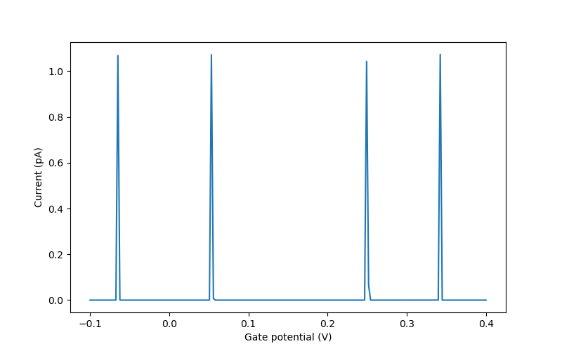
Fig. 6.4.9 Coulomb peaks with respect to reference gate potential (see the note in Creating the junction, above).

6.5. Computing the charge-stability diagram

As a second example for the seq_tunnel_curr method, we compute the charge-stability diagram of our quantum dot. The first step is to define the grid of plunger gate and drain potentials (respectively, v_gate_rng and v_drain_rng) over which we will sample the charge current.

### Charge-stability diagram ###
v_gate_rng = np.linspace(-0.2, 0.5, num=200)
v_drain_rng = np.linspace(-0.02, 0.02, num=50)

We then define diam, the array in which we will store the charge current. Its dimensions are v_gate_rng.size by v_drain_rng.size: the current will be computed for all pairs consisting in one element of v_gate_rng.size and one element of v_drain_rng.size.

diam = np.zeros((v_gate_rng.size,v_drain_rng.size), dtype=float)

Note that the data type of the elements of diam is specified to be dtype=float.

Since the master-equation calculation will be performed for each element of diam, we initialize a progress bar. The argument max = number_grid_points specifies the total number of such calculations.

number_grid_points = v_gate_rng.size * v_drain_rng.size # number of sampled grid points
progress_bar = Bar("Computing charge-stability diagram", max = number_grid_points) # initialize progress bar

Next, we iterate over all elements of v_gate_rng, adjusting the gate potential of the junction jc using the setVg method.

for i in range(v_gate_rng.size):        # loop over gate voltage
    v_gate = v_gate_rng[i]
    jc.setVg(v_gate)

We perform a nested iteration over the elements of v_drain_rng, adjusting the drain potentials using the setVd methods, computing the source current using the seq_tunnel_curr method, and storing the result, Il, into diam. To denote the progress of the calculation on the progress bar, the next() method is called on progress_bar at the end of each iteration of the inner loop.

for j in range(v_drain_rng.size):      # loop over drain voltage
    v_drain = v_drain_rng[j]
    jc.setVd(v_drain)
    Il,Ir,prob = seq_tunnel_curr(jc)    # transport calculation
    diam[i,j] = Il
    progress_bar.next()

Once the calculations performed using the nested for loops are done, we call the finish() method on progress_bar.

progress_bar.finish()

We then postprocess the current to turn it into an image to be plotted.

# Postprocess the current to turn it into an image to be plotted
current_image = np.flip(np.transpose(np.abs(diam)), axis=0)

Finally, this current is plotted on a color plot and saved as stability.png.

# plot results
fig, axs = plt.subplots()
axs.set_ylabel('$V_d(V)$',fontsize=16)
axs.set_xlabel('$V_g(V)$',fontsize=16)
diff_cond_map = axs.imshow(current_image/1e-12, interpolation='bilinear',
        extent=[Vtop_2+v_gate_rng[0], Vtop_2+v_gate_rng[-1],
                v_drain_rng[0], v_drain_rng[-1]], aspect="auto", cmap="Reds")
fig.colorbar(diff_cond_map, ax=axs, label="Current (pA)")
fig.tight_layout()
path_fig = str(script_dir/"output"/"stability.png")
plt.savefig(path_fig)
plt.show()

This results in the following diagram, which displays the Coulomb diamonds structure expected for a quantum dot.

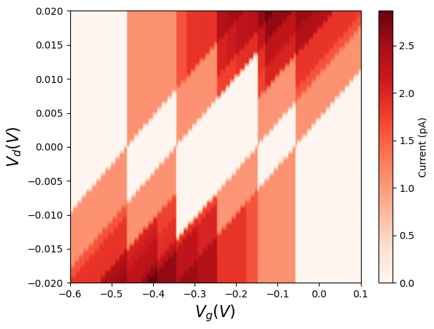
Fig. 6.5.1 Charge-stability diagram with respect to reference gate potential (see the note in Creating the junction, above).

Note

Please refer to the Quantum transport—Master equation tutorial for an explanation of how to calculate and plot the differential conductance.

6.6. Full code

__copyright__ = "Copyright 2023, Nanoacademic Technologies Inc."

import numpy as np
import pathlib
from matplotlib import pyplot as plt
import pickle
from progress.bar import ChargingBar as Bar
from device import constants as ct
from device.mesh3d import Mesh, SubMesh
from device import io
from device import Device, SubDevice
from device.schrodinger import Solver
from device.many_body import SolverParams
from transport.mastereq import seq_tunnel_curr
from transport.junction import Junction
from device import materials as mt

# Load the mesh
script_dir = pathlib.Path(__file__).parent.resolve()
path_mesh = str(script_dir/'meshes'/'gated_dot.msh2')
scaling = 1e-6
mesh = Mesh(scaling, path_mesh)

# Create device
d = Device(mesh, conf_carriers="e")
d.set_temperature(0.1)

# # Applied potentials
Vtop_1 = -0.5
Vtop_2 = -0.4
Vtop_3 = -0.5
Vbottom_1 = -0.5
Vbottom_2 = -0.4
Vbottom_3 = -0.5

# Work function of the metallic gates at midgap of GaAs
barrier = 0.834*ct.e    # n-type Schottky barrier height

# Ionized dopant density
doping = 3e18*1e6   # In SI units

# Set up materials in heterostructure stack
d.new_region("cap", mt.GaAs)
d.new_region("barrier", mt.AlGaAs)
d.new_region("dopant_layer", mt.AlGaAs,ndoping=doping)
d.new_region("spacer_layer", mt.AlGaAs)
d.new_region("spacer_dot", mt.AlGaAs)
d.new_region("two_deg", mt.GaAs)
d.new_region("two_deg_dot", mt.GaAs)
d.new_region("substrate", mt.GaAs)
d.new_region("substrate_dot", mt.GaAs)

# Remove unphysical charge from cap and barrier
d.new_insulator("cap")
d.new_insulator("barrier")

# Align the bands across hetero-interfaces using GaAs as the reference material
d.align_bands(mt.GaAs)

# Set up boundary conditions
d.new_schottky_bnd("top_gate_1", Vtop_1, barrier)
d.new_schottky_bnd("top_gate_2", Vtop_2, barrier)
d.new_schottky_bnd("top_gate_3", Vtop_3, barrier)
d.new_schottky_bnd("bottom_gate_1", Vbottom_1, barrier)
d.new_schottky_bnd("bottom_gate_2", Vbottom_2, barrier)
d.new_schottky_bnd("bottom_gate_3", Vbottom_3, barrier)
d.new_ohmic_bnd("ohmic_bnd")

# Load the confinement potential from previous run
path_in = str(script_dir/"output"/"electric_potential_-0.400V.hdf5")
d.set_potential(io.load(path_in))

# Create a submesh in which to solve Schrodinger's equation
submesh = SubMesh(mesh, ["spacer_dot","two_deg_dot","substrate_dot"])

# Create subdevice
subdevice = SubDevice(d, submesh)

# Solver the single-electron problem to get basis set
slv = Solver(subdevice)
slv.solve()
subdevice.print_energies()

many_body_solver_params = SolverParams()
many_body_solver_params.num_states = 2  # Number of levels to keep
many_body_solver_params.n_degen = 2     # spin degenerate system
many_body_solver_params.alpha = 0.0714  # lever arm
jc = Junction(subdevice, many_body_solver_params=many_body_solver_params)

print('chemical potentials (eV):', jc.chem_potentials/ct.e)
print('positions of Coulomb peaks relative to reference value (V):',
    jc.coulomb_peak_pos)

# Set a near-zero source-drain bias
jc.setVs(0.0001)
jc.setVd(-0.0001)

jc.set_source_broad_func(10e6)
jc.set_drain_broad_func(10e6)

v_gate_rng = np.linspace(-0.1, 0.4, num=200)

# Calculate the current for each plunger gate potential
vec_Il = []
for i in range(v_gate_rng.size):        # loop over gate voltage
    v_gate = v_gate_rng[i]
    jc.setVg(v_gate)
    Il,Ir,prob = seq_tunnel_curr(jc)    # transport calculation
    vec_Il += [Il]

path_out = str(script_dir/'output'/'current.pkl')
outfile = open(path_out, 'wb')
pickle.dump((v_gate_rng,vec_Il), outfile)
outfile.close()

fig = plt.figure(figsize=(8,5))
ax = fig.add_subplot(1,1,1)
ax.set_xlabel("Gate potential (V)")
ax.set_ylabel("Current (pA)")
ax.plot(v_gate_rng, np.array(vec_Il)/1e-12)
path_fig = str(script_dir/"output"/"coulomb_peaks.png")
plt.savefig(path_fig)
plt.show()

### Charge-stability diagram ###
v_gate_rng = np.linspace(-0.2, 0.5, num=200)
v_drain_rng = np.linspace(-0.02, 0.02, num=50)

diam = np.zeros((v_gate_rng.size,v_drain_rng.size), dtype=float)

number_grid_points = v_gate_rng.size * v_drain_rng.size # number of sampled grid points
progress_bar = Bar("Computing charge-stability diagram", max = number_grid_points) # initialize progress bar

for i in range(v_gate_rng.size):        # loop over gate voltage
    v_gate = v_gate_rng[i]
    jc.setVg(v_gate)

    for j in range(v_drain_rng.size):      # loop over drain voltage
        v_drain = v_drain_rng[j]
        jc.setVd(v_drain)
        Il,Ir,prob = seq_tunnel_curr(jc)    # transport calculation
        diam[i,j] = Il
        progress_bar.next()

progress_bar.finish()

# Postprocess the current to turn it into an image to be plotted
current_image = np.flip(np.transpose(np.abs(diam)), axis=0)

# plot results
fig, axs = plt.subplots()
axs.set_ylabel('$V_d(V)$',fontsize=16)
axs.set_xlabel('$V_g(V)$',fontsize=16)
diff_cond_map = axs.imshow(current_image/1e-12, interpolation='bilinear',
        extent=[Vtop_2+v_gate_rng[0], Vtop_2+v_gate_rng[-1],
                v_drain_rng[0], v_drain_rng[-1]], aspect="auto", cmap="Reds")
fig.colorbar(diff_cond_map, ax=axs, label="Current (pA)")
fig.tight_layout()
path_fig = str(script_dir/"output"/"stability.png")
plt.savefig(path_fig)
plt.show()