5. Calculating the Coulomb peaks of a quantum dot

5.1. Requirements

5.1.1. Software components

• QTCAD

5.1.2. Mesh file

• qtcad/examples/practical_application/meshes/gated_dot.msh

5.1.3. Python script

• qtcad/examples/practical_application/5-many_body.py

5.1.4. References

• Calculating the lever arm of a quantum dot

• Many-body solver

5.2. Briefing

In this previous tutorial, we computed the lever arm of a quantum dot. Transport in a quantum dot is characterized by a phenomenon known as Coulomb blockade. Specifically, only an integer number of electrons can reside in the quantum dot. When a chemical potential of the dot lies between the source and drain chemical potentials, the number of electrons in the dot can fluctuate between \(N-1\) and \(N\) (where \(N\) is an integer), resulting in finite conductance. On the other hand, when there are no chemical potentials between the source and drain chemical potentials, the number of electrons cannot fluctuate between two integer values, resulting is zero conductance. These chemical potentials—i.e., the difference in total energy between a quantum dot with \(N-1\) and \(N\) electrons in their ground state (see Chemical potentials)—therefore play a crucial role in transport in this device. The Coulomb peaks, i.e. local maximums in the dot conductivity with respect to an applied gate potential, are related to the chemical potentials and the lever arm (see Coulomb peak positions).

In this tutorial, we will compute the chemical potentials and Coulomb peaks of the quantum dot of the previous tutorials at a value of the plunger gates potential of \(-0.4\textrm{ V}\), which approximately corresponds to the gate bias at which the quantum-dot ground state energy (which is equal to the chemical potential with \(N=1\)) crosses the Fermi level (set to zero by convention in QTCAD).

5.3. Setting up the device

5.3.1. Header

We start by importing relevant modules.

import pathlib
import numpy as np

from qtcad.device.mesh3d import Mesh, SubMesh
from qtcad.device import io
from qtcad.device import constants as ct

from qtcad.device import materials as mt
from qtcad.device import Device, SubDevice
from qtcad.device.schrodinger import Solver as SingleBodySolver
from qtcad.device.many_body import Solver as ManyBodySolver
from qtcad.device.many_body import SolverParams

These modules were described in the previous tutorials with the exception of many_body, which is used to define and solve the many-body problem of \(N\) interacting electrons in a device.

5.3.2. Defining the device and its electric potential

We start by defining the device as was previously done. Note that the plunger gates potentials, Vtop_2 and Vbottom_2, are set to -0.4.

# Load the mesh
script_dir = pathlib.Path(__file__).parent.resolve()
path_mesh = str(script_dir /'meshes'/'gated_dot.msh')
scaling = 1e-6
mesh = Mesh(scaling, path_mesh)

# Create device
d = Device(mesh, conf_carriers="e")
d.set_temperature(0.1)

# # Applied potentials
Vtop_1 = -0.5
Vtop_2 = -0.4
Vtop_3 = -0.5
Vbottom_1 = -0.5
Vbottom_2 = -0.4
Vbottom_3 = -0.5

# Work function of the metallic gates at midgap of GaAs
barrier = 0.834*ct.e    # n-type Schottky barrier height

# Ionized dopant density
doping = 3e18*1e6   # In SI units

# Set up materials in heterostructure stack
d.new_region("cap", mt.GaAs)
d.new_region("barrier", mt.AlGaAs)
d.new_region("dopant_layer", mt.AlGaAs,ndoping=doping)
d.new_region("spacer_layer", mt.AlGaAs)
d.new_region("spacer_dot", mt.AlGaAs)
d.new_region("two_deg", mt.GaAs)
d.new_region("two_deg_dot", mt.GaAs)
d.new_region("substrate", mt.GaAs)
d.new_region("substrate_dot", mt.GaAs)

# Remove unphysical charge from cap and barrier
d.new_insulator("cap")
d.new_insulator("barrier")

# Align the bands across hetero-interfaces using GaAs as the reference material
d.align_bands(mt.GaAs)

# Set up boundary conditions
d.new_schottky_bnd("top_gate_1", Vtop_1, barrier)
d.new_schottky_bnd("top_gate_2", Vtop_2, barrier)
d.new_schottky_bnd("top_gate_3", Vtop_3, barrier)
d.new_schottky_bnd("bottom_gate_1", Vbottom_1, barrier)
d.new_schottky_bnd("bottom_gate_2", Vbottom_2, barrier)
d.new_schottky_bnd("bottom_gate_3", Vbottom_3, barrier)
d.new_ohmic_bnd("ohmic_bnd")

The next step is to set the electric potential in the device. This could be done by solving the nonlinear Poisson equation, as has been done in previous tutorials. However, here, we simply load this potential from the relevant .hdf5 file generated in Calculating the lever arm of a quantum dot, which is set as the device potential saved in d.phi. Remark that the method set_potential also automatically calls set_V_from_phi to update the confinement potential accordingly.

# Load the confinement potential from previous run
path_in = str(script_dir/"output"/"electric_potential_-0.400V.hdf5")
d.set_potential(io.load(path_in))

5.4. Solving Schrödinger’s equation

Next, Schrödinger’s equation is solved using the usual method.

# Create a submesh in which to solve Schrodinger's equation
submesh = SubMesh(mesh, ["spacer_dot","two_deg_dot","substrate_dot"])

# Create subdevice
subdevice = SubDevice(d, submesh)

# Solve the single-electron problem to get basis set
slv = SingleBodySolver(subdevice)
slv.solve()
subdevice.print_energies()

In this case, the energy levels are as follows.

Energy levels (eV)
[-0.00461879  0.00569634  0.00997394  0.01614266  0.02039089  0.02510846
  0.02715079  0.03101003  0.03571226  0.03786466]

As a sanity check, we visualize the confining potential and the eigenfunctions of the ground state and the first two excited states.

# Plot the first few envelope functions
from device import analysis as an
an.plot_slices(submesh,subdevice.V/ct.e,title="Confinement potential")
an.plot_slices(submesh,subdevice.eigenfunctions[:,0],title="Ground state")
an.plot_slices(submesh,subdevice.eigenfunctions[:,1],title="1st excited state")
an.plot_slices(submesh,subdevice.eigenfunctions[:,2],title="2nd excited state")

This results in the following figures.

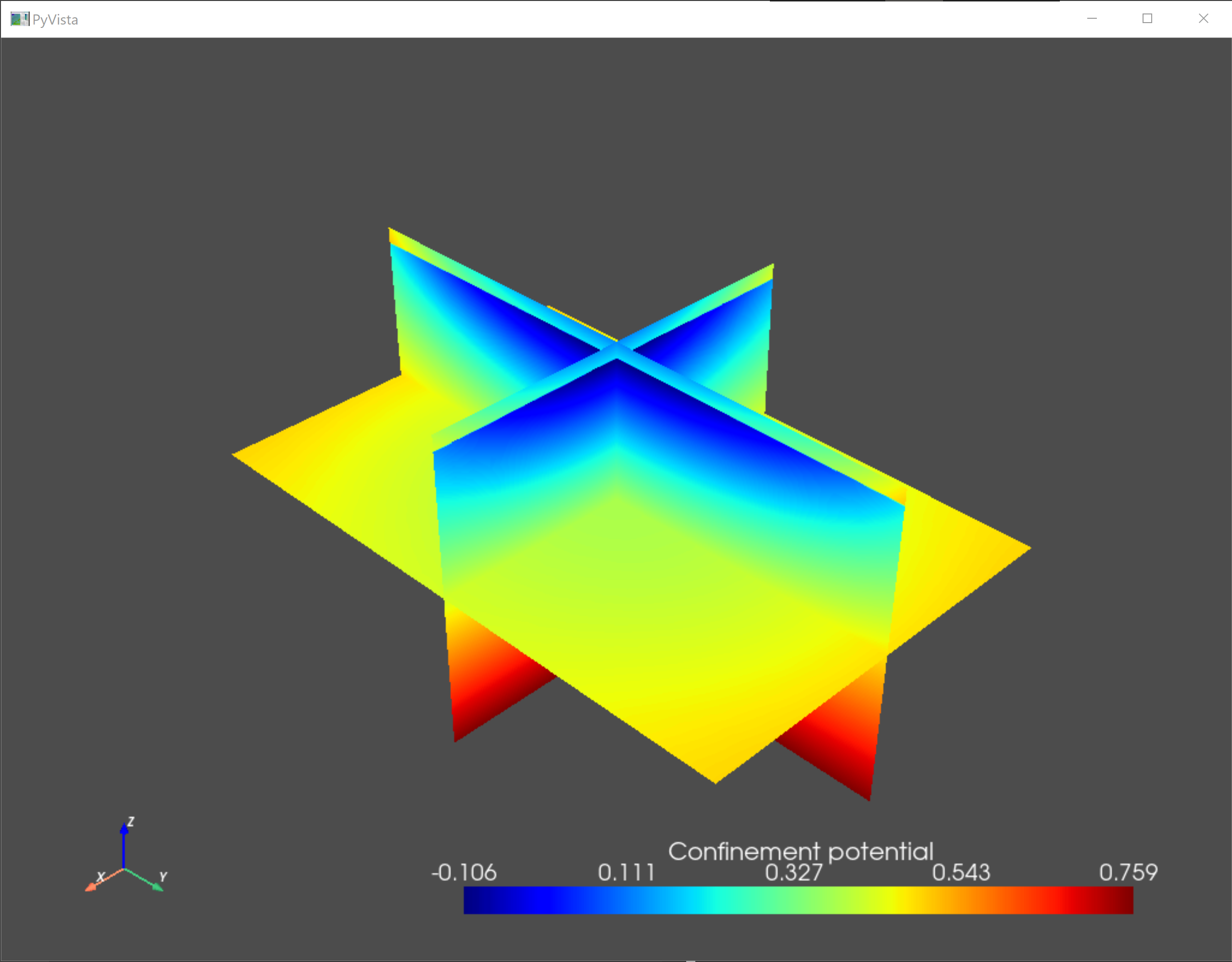
Fig. 5.4.1 Confinement potential

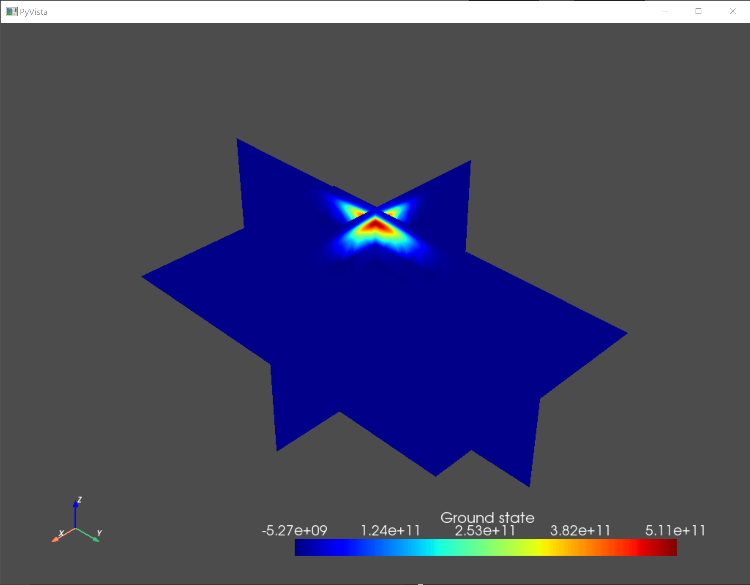
Fig. 5.4.2 Ground state

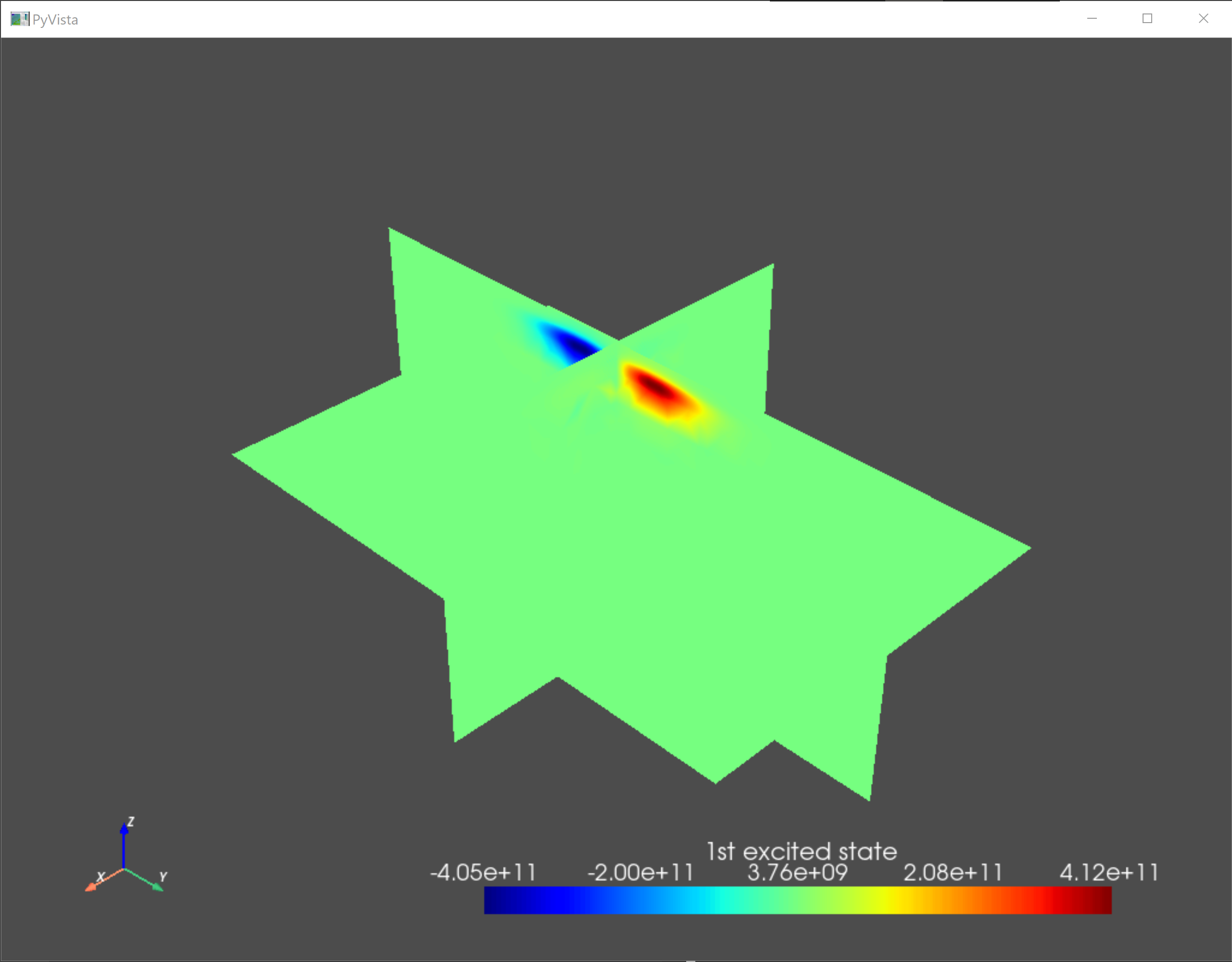
Fig. 5.4.3 First excited state

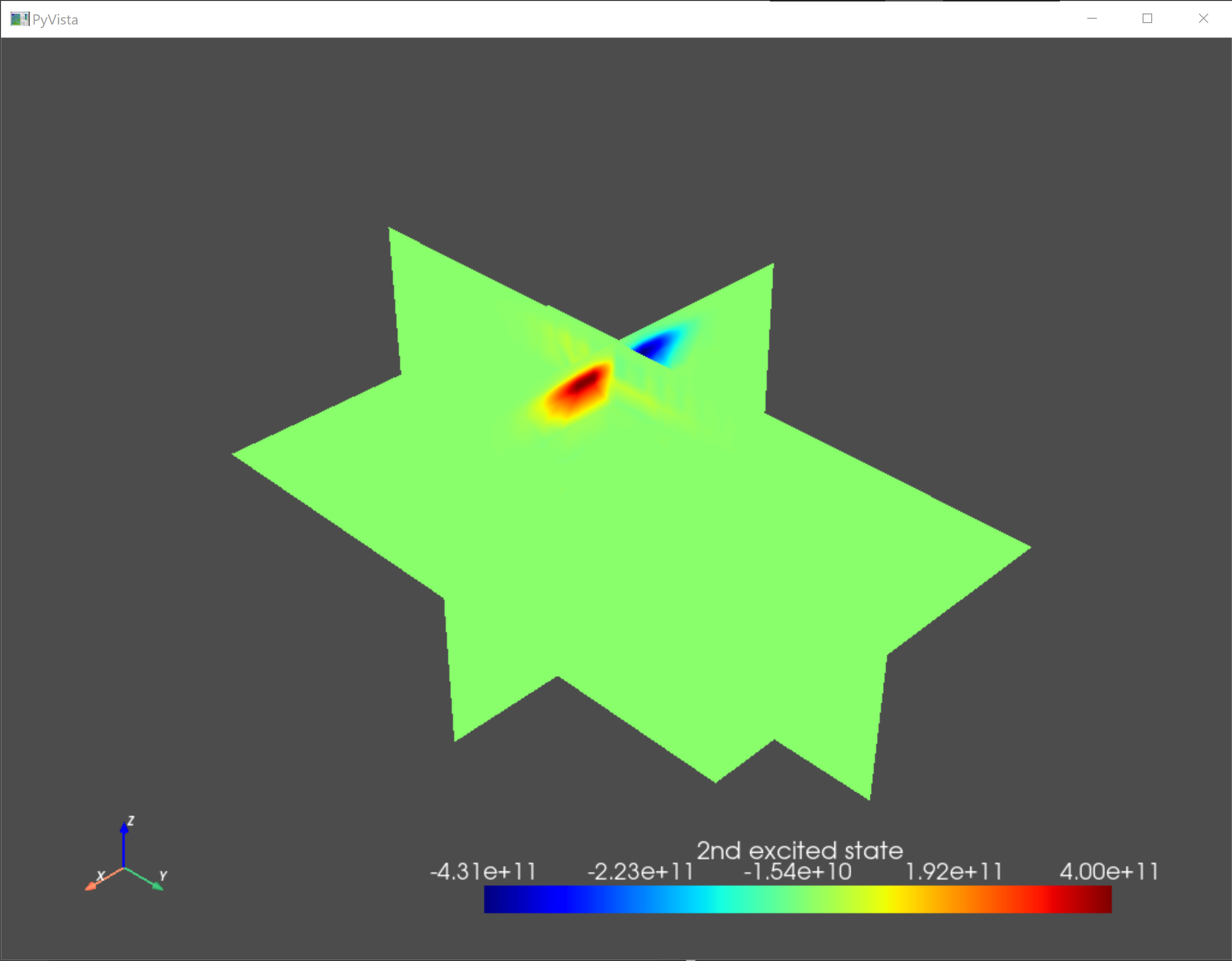
Fig. 5.4.4 Second excited state

5.5. Setting up the many-body solver and calculating the Coulomb peaks

We are now ready to define a many-body Solver object, and run it with:

# Create the many-body solver and call its solve method
solver_params = SolverParams()
solver_params.num_states = 3    # Number orbital basis states to consider
solver_params.n_degen = 2       # spin degenerate system
solver_params.alpha = 0.0714     # Lever arm
slv = ManyBodySolver(subdevice, solver_params = solver_params)
slv.solve()

The first argument of the many-body Solver object constructor is subdevice, and corresponds to the subdevice object of the quantum dot. As an optional argument, we also provide a SolverParams object, in which we modified three solver paramaters. The first, num_states specifies that only the three lowest energy levels in the quantum dot should be considered. Solving the many-body problem involves the calculation of numerous Coulomb integrals; the number of these integrals scales with the fourth power of the number of energy levels. The second, n_degen, describes the degeneracy of the dot’s eigenstates. Since our system is spin-degenerate, this argument is equal to \(2\). The third, alpha is the lever arm which we computed in the previous tutorial.

At this point, the calculation of Coulomb integrals begins; these integrals describe the Coulomb interactions between electrons in the dot.

Computing Coulomb integrals ███∙∙∙∙∙∙∙∙∙∙∙∙∙∙∙∙∙∙∙∙∙∙∙∙∙∙∙∙∙ 12%

This calculation may take up to a few minutes to run, after which the resulting many-body Hamiltonian is diagonalized and the results are stored in the subdevice object. After this, we can print and save the chemical potentials and Coulomb peaks.

# Output positions of chemical potentials and Coulomb peaks
path_chem_potentials = str(script_dir/"output"/"chem_potentials.txt")
path_peak_pos = str(script_dir/"output"/"peak_positions.txt")
print('chemical potentials (eV):', subdevice.chem_potentials/ct.e)
np.savetxt(path_chem_potentials,subdevice.chem_potentials/ct.e)
print('positions of Coulomb peaks relative to reference value (V):',
    subdevice.coulomb_peak_pos)
np.savetxt(path_peak_pos,subdevice.coulomb_peak_pos)

The chem_potentials attribute of the subdevice corresponds to the list of chemical potentials obtained by running the many-body solver, while the coulomb_peak_pos attribute corresponds to the Coulomb peaks. This should result in the following.

chemical potentials (eV): [-0.00461879  0.00376343  0.01784489  0.02440783  0.03394929  0.04072094]
positions of Coulomb peaks relative to reference value (V): [-0.06468898  0.05270916  0.24992838  0.34184641
0.47548022  0.57032126]

Note

The position of the Coulomb peaks is given relative to the reference gate potential. The reference gate potential is the potential applied at the boundary condition when solving Poisson’s equation. Here, this reference potential is Vtop_2 = Vbottom_2 = -0.4 V, so that this value should be added to the above peak positions to find the true potentials to be applied at the gates to observe transport.

5.6. Full code

__copyright__ = "Copyright 2024, Nanoacademic Technologies Inc."

import pathlib
import numpy as np
from qtcad.device.mesh3d import Mesh, SubMesh
from qtcad.device import io
from qtcad.device import constants as ct
from qtcad.device import materials as mt
from qtcad.device import Device, SubDevice
from qtcad.device.schrodinger import Solver as SingleBodySolver
from qtcad.device.many_body import Solver as ManyBodySolver
from qtcad.device.many_body import SolverParams

# Load the mesh
script_dir = pathlib.Path(__file__).parent.resolve()
path_mesh = str(script_dir /'meshes'/'gated_dot.msh')
scaling = 1e-6
mesh = Mesh(scaling, path_mesh)

# Create device
d = Device(mesh, conf_carriers="e")
d.set_temperature(0.1)

# # Applied potentials
Vtop_1 = -0.5
Vtop_2 = -0.4
Vtop_3 = -0.5
Vbottom_1 = -0.5
Vbottom_2 = -0.4
Vbottom_3 = -0.5

# Work function of the metallic gates at midgap of GaAs
barrier = 0.834*ct.e    # n-type Schottky barrier height

# Ionized dopant density
doping = 3e18*1e6   # In SI units

# Set up materials in heterostructure stack
d.new_region("cap", mt.GaAs)
d.new_region("barrier", mt.AlGaAs)
d.new_region("dopant_layer", mt.AlGaAs,ndoping=doping)
d.new_region("spacer_layer", mt.AlGaAs)
d.new_region("spacer_dot", mt.AlGaAs)
d.new_region("two_deg", mt.GaAs)
d.new_region("two_deg_dot", mt.GaAs)
d.new_region("substrate", mt.GaAs)
d.new_region("substrate_dot", mt.GaAs)

# Remove unphysical charge from cap and barrier
d.new_insulator("cap")
d.new_insulator("barrier")

# Align the bands across hetero-interfaces using GaAs as the reference material
d.align_bands(mt.GaAs)

# Set up boundary conditions
d.new_schottky_bnd("top_gate_1", Vtop_1, barrier)
d.new_schottky_bnd("top_gate_2", Vtop_2, barrier)
d.new_schottky_bnd("top_gate_3", Vtop_3, barrier)
d.new_schottky_bnd("bottom_gate_1", Vbottom_1, barrier)
d.new_schottky_bnd("bottom_gate_2", Vbottom_2, barrier)
d.new_schottky_bnd("bottom_gate_3", Vbottom_3, barrier)
d.new_ohmic_bnd("ohmic_bnd")

# Load the confinement potential from previous run
path_in = str(script_dir/"output"/"electric_potential_-0.400V.hdf5")
d.set_potential(io.load(path_in))

# Create a submesh in which to solve Schrodinger's equation
submesh = SubMesh(mesh, ["spacer_dot","two_deg_dot","substrate_dot"])

# Create subdevice
subdevice = SubDevice(d, submesh)

# Solve the single-electron problem to get basis set
slv = SingleBodySolver(subdevice)
slv.solve()
subdevice.print_energies()

# Plot the first few envelope functions
from device import analysis as an
an.plot_slices(submesh,subdevice.V/ct.e,title="Confinement potential")	
an.plot_slices(submesh,subdevice.eigenfunctions[:,0],title="Ground state")	
an.plot_slices(submesh,subdevice.eigenfunctions[:,1],title="1st excited state")	
an.plot_slices(submesh,subdevice.eigenfunctions[:,2],title="2nd excited state")

# Create the many-body solver and call its solve method
solver_params = SolverParams()
solver_params.num_states = 3    # Number orbital basis states to consider
solver_params.n_degen = 2       # spin degenerate system
solver_params.alpha = 0.0714     # Lever arm
slv = ManyBodySolver(subdevice, solver_params = solver_params)
slv.solve()

# Output positions of chemical potentials and Coulomb peaks
path_chem_potentials = str(script_dir/"output"/"chem_potentials.txt")
path_peak_pos = str(script_dir/"output"/"peak_positions.txt")
print('chemical potentials (eV):', subdevice.chem_potentials/ct.e)
np.savetxt(path_chem_potentials,subdevice.chem_potentials/ct.e)
print('positions of Coulomb peaks relative to reference value (V):',
    subdevice.coulomb_peak_pos)
np.savetxt(path_peak_pos,subdevice.coulomb_peak_pos)