3. Simulating bound states in a quantum dot using the quantum-well and Schrödinger solvers
3.1. Requirements
3.1.1. Software components
QTCAD
devicegen
3.1.2. Mesh file
qtcad/examples/practical_application/meshes/gated_dot.msh
3.1.3. Python script
qtcad/examples/practical_application/3-QW_schrodinger.py
3.1.4. References
3.2. Briefing
In the previous tutorial, we have used the nonlinear Poisson solver to obtain the confinement potential in our gated quantum dot. We have then used the Schrödinger solver to obtain this quantum dot’s eigenspectrum. In this approach, we have separated the simulation domain into two regions. The first region consisted of a small “quantum dot” region in which no classical charge is considered, and confinement was fully modeled along all directions. The second region consisted of all volumes that surround the quantum dot—in this region, no quantum confinement was considered and charge densities were calculated from equilibrium statistical mechanics assuming that electrons in the conduction and valence bands occupied plane-wave states (see the Carrier statistics theory section). Since the quantum dot forms at an interface that is only a few nanometers thick (the 2DEG at the AlGaAs–GaAs heterojunction), this approach suffers from a conceptual shortcoming: it ignores the effect of quantum confinement along the \(z\) direction (namely, the heterostructure growth direction) in the classical charge reservoirs that surround the quantum dot.
To resolve this conceptual issue, in this tutorial, we will obtain the gated quantum dot’s confinement potential via the quantum-well solver. This solver assumes a strong quantum confinement along one direction (here, the \(z\) direction) and quasi-translational invariance along the two other directions (here, the \(x\) and \(y\) directions). Specifically, with the quantum well solver, the density of confined carriers is computed as follows:
define 2D coordinates \(\left(x_i, y_i\right)\), \(i=1,\cdots,N\), of \(N\) linecuts parallel to the \(z\) axis;
solve 1D Schrödinger equations on the \(N\) linecuts;
compute the charge density in the neighborhood of each of the \(N\) linecuts by assuming the wavefunctions is described by plane waves along the \(x\) and \(y\) directions, i.e., through (7.17);
interpolate the charge density between the linecuts.
The charge density and electric potential are computed self-consistently in the quantum-well solver, as in the Schrödinger–Poisson solver. The full theoretical details of the quantum-well solver are described in Carrier densities in nearly-translationally-invariant systems.
Once we have obtained the confinement potential, we will compute the dot’s energy levels using the Schrödinger solver. Throughout this tutorial, we will investigate the main qualitative differences between the outputs of the nonlinear Poisson and quantum-well solvers.
3.3. Setting up the device
3.3.1. Header
We start by importing the relevant modules.
from qtcad.device import constants as ct
from qtcad.device.mesh3d import Mesh, SubMesh
from qtcad.device import io
from qtcad.device import materials as mt
from qtcad.device import Device, SubDevice
from qtcad.device.quantum_well import Solver as QuantumWellSolver
from devicegen import DeviceGenerator
from qtcad.device.mesh2d import Mesh as Mesh2D
from qtcad.device.schrodinger import Solver as SchrodingerSolver
from qtcad.device.poisson import SolverParams as PoissonSolverParams
from qtcad.device.schrodinger import SolverParams as SchrodingerSolverParams
from qtcad.device.quantum_well import SolverParams as QuantumWellSolverParams
import pathlib
These modules were all used in the previous tutorial, with the following exceptions:
QuantumWellSolver: The quantum-well solver, used to obtain the electric potential throughout the entire device, and thus the confinement potential for the quantum dot, in a way that accounts for quantum confinement along the heterostructure growth axis.DeviceGeneratorandMesh2D: These classes will be used to generate the linecut positions from the gate layout file for the quantum-well solver.QuantumWellSolverParams: The solver parameters for the quantum-well solver.
3.3.2. Loading the mesh, defining material composition, and applying external voltages
In the following, we define the device and external voltages in the exact same way as in the previous tutorial.
# Input file
script_dir = pathlib.Path(__file__).parent.resolve()
path_mesh = str(script_dir/'meshes'/'gated_dot.msh')

# Load the mesh
scaling = 1e-6
mesh = Mesh(scaling,path_mesh)
mesh.show()

# Create device
d = Device(mesh, conf_carriers="e")
d.set_temperature(0.1)

# Ionized dopant density
doping = 3e18*1e6   # In SI units

# Set up materials in heterostructure stack
d.new_region("cap", mt.GaAs)
d.new_region("barrier", mt.AlGaAs)
d.new_region("dopant_layer", mt.AlGaAs,ndoping=doping)
d.new_region("spacer_layer", mt.AlGaAs)
d.new_region("spacer_dot", mt.AlGaAs)
d.new_region("two_deg", mt.GaAs)
d.new_region("two_deg_dot", mt.GaAs)
d.new_region("substrate", mt.GaAs)
d.new_region("substrate_dot", mt.GaAs)

# Align the bands across hetero-interfaces using GaAs as the reference material
d.align_bands(mt.GaAs)

# Remove unphysical charge from cap and barrier
d.new_insulator("cap")
d.new_insulator("barrier")

# Applied potentials
Vtop_1 = -0.5
Vtop_2 = -0.5
Vtop_3 = -0.5
Vbottom_1 = -0.5
Vbottom_2 = -0.5
Vbottom_3 = -0.5

# Work function of the metallic gates at midgap of GaAs
barrier = 0.834*ct.e    # n-type Schottky barrier height

# Set up boundary conditions
d.new_schottky_bnd("top_gate_1", Vtop_1, barrier)
d.new_schottky_bnd("top_gate_2", Vtop_2, barrier)
d.new_schottky_bnd("top_gate_3", Vtop_3, barrier)
d.new_schottky_bnd("bottom_gate_1", Vbottom_1, barrier)
d.new_schottky_bnd("bottom_gate_2", Vbottom_2, barrier)
d.new_schottky_bnd("bottom_gate_3", Vbottom_3, barrier)
d.new_ohmic_bnd("ohmic_bnd")
3.4. Solving for the electric potential using the quantum-well solver
Now that the device has been set up, we will compute the confinement potential
of the quantum dot using the quantum-well solver. As for the nonlinear Poisson
solver, to avoid significant screening in the quantum dot region, we set the
charge in the quantum dot region to zero using the
set_dot_region method.
# Create a submesh including only the dot region
submesh_qd = SubMesh(mesh, ["spacer_dot","two_deg_dot","substrate_dot"])
submesh_qd.show()

# Set up the dot region in which no charge is allowed in the quantum-well solver
d.set_dot_region(submesh_qd)
The next step is to set up the
QuantumWellSolver object. For this,
we start by a creating a subdevice corresponding to the quantum well region,
in which 1D Schrödinger equations will be solved.
# Create subdevice for the quantum well region
submesh_qw = SubMesh(mesh, ["spacer_layer", "spacer_dot", "two_deg", "two_deg_dot", "substrate", "substrate_dot"])
submesh_qw.show()
qw_subdevice = SubDevice(d, submesh_qw)
The quantum charge will thus be limited to lie within qw_subdevice by the
quantum-well solver. Outside qw_subdevice, the quantum-well solver
computes the charge classically. To ensure a proper quantum-mechanical
treatment of the charge in the 2DEG, the quantum well region should be made
large enough (in particular, the region should straddle interfaces that play
a role in quantum confinement of the 2DEG). Here, we include the spacer, and
substrate layers within qw_subdevice.
We then define solver parameters for the quantum-well solver. Much like in the
Schrödinger–Poisson solver, the quantum-well solver solves Schrödinger and
Poisson equations iteratively until self-consistency is reached. Hence, three
sets of solver parameters are required: one for the Poisson equation
(poisson_params), one for the Schrödinger equation (schrod_params), and
one for the coupled Schrödinger–Poisson equations (qw_params).
# Solver parameters for the quantum-well solver
poisson_params = PoissonSolverParams()
schrod_params = SchrodingerSolverParams({"ti_directions": ["x", "y"]})
qw_params = QuantumWellSolverParams()
qw_params.poisson_solver_params = poisson_params
qw_params.schrod_solver_params = schrod_params
Here, we have simply used the default solver parameters values, except for
the ti_directions attribute of the Schrödinger solver parameters
(schrod_params), which we have set to ["x", "y"]. This imposes
quasi-translational invariance along the \(x\) and \(y\) directions for
the purpose of computing 3D charge density from 1D envelope functions (through
(7.17)).
Finally, we create a set of 2D coordinates defining linecuts parallel to the
\(z\) axis on which 1D Schrödinger equations will be solved in the
quantum-well solver. To do so, we employ devicegen and simply define a 2D mesh
based on the gate layout, which we store in the variable mesh_2d.
# define coordinates for linecuts through the quantum well using devicegen
char_len = 20 * 1e-3
path_layout = str(script_dir / "layouts" / "gated_qd.txt")
path_geo_2d = str(script_dir / "layouts" / "gated_qd_2d.geo")
dG = DeviceGenerator(path_layout, outfile=path_geo_2d, h=char_len)
path_mesh_2d = str(script_dir / "meshes" / "gated_qw_2d.msh")
dG.save_mesh(mesh_name=path_mesh_2d)
mesh_2d = Mesh2D(scaling, path_mesh_2d)
mesh_2d.show()
Below, we show the resulting 2D mesh.
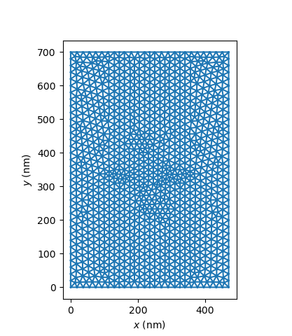
Fig. 3.4.2 Positions of linecuts for the quantum-well solver
We are now ready to instantiate the quantum-well solver object.
# Set up quantum-well solver
qw_solver = QuantumWellSolver(
    d=d, qw_subdevice=qw_subdevice, coords=mesh_2d, solver_params=qw_params
    )
The electric potential in the device d, which will define the confining
potential for the quantum dot, may then be obtained as follows.
# Solve
qw_solver.solve()
Quantum-well solver simulations are computationally heavier than basic non-linear Poisson simulations; this particular simulation may take a few minutes to run on a typical laptop. You may notice the following log line near the beginning of the simulation:
Preparing Quantum Well Solver
This line simply indicates that some pre-self-consistent-simulation steps are being performed, e.g. the instantiation of the linecuts used by the quantum-well solver. For simulations with a very dense 3D device mesh and/or a very dense 2D linecut coordinates mesh, this step may take a long time.
The next line in the log, i.e.,
INITIALIZING FROM NON-LINEAR POISSON EQUATION
simply indicates that the device potential is computed from the nonlinear Poisson equation, as an initial guess for the coupled Schrödinger–Poisson equations used in the rest of the quantum-well solver.
Finally, the log following
LAUNCHING SELF-CONSISTENT SCHRODINGER-POISSON LOOP
provides information about the computation time, maximum error, and convergence status of the coupled Schrödinger–Poisson equations for the quantum-well solver.
After the quantum-well solver converges, the results are saved in .vtu
files for visualization.
# Save the conduction band edge in .vtu format
outfile_cond_band_edge = str(script_dir / "output" / "cond_band_edge_qw.vtu")
out_dict = {"EC (eV)": d.cond_band_edge()/ct.e}
io.save(outfile_cond_band_edge, out_dict, mesh)

# Save the electron density in .vtu format
outfile_electron_dens = str(script_dir / "output" / "electron_dens_qw.vtu")
out_dict = {"n (1/m^3)": d.n}
io.save(outfile_electron_dens, out_dict, mesh)
For example, the figure below shows a side view of the electron density.
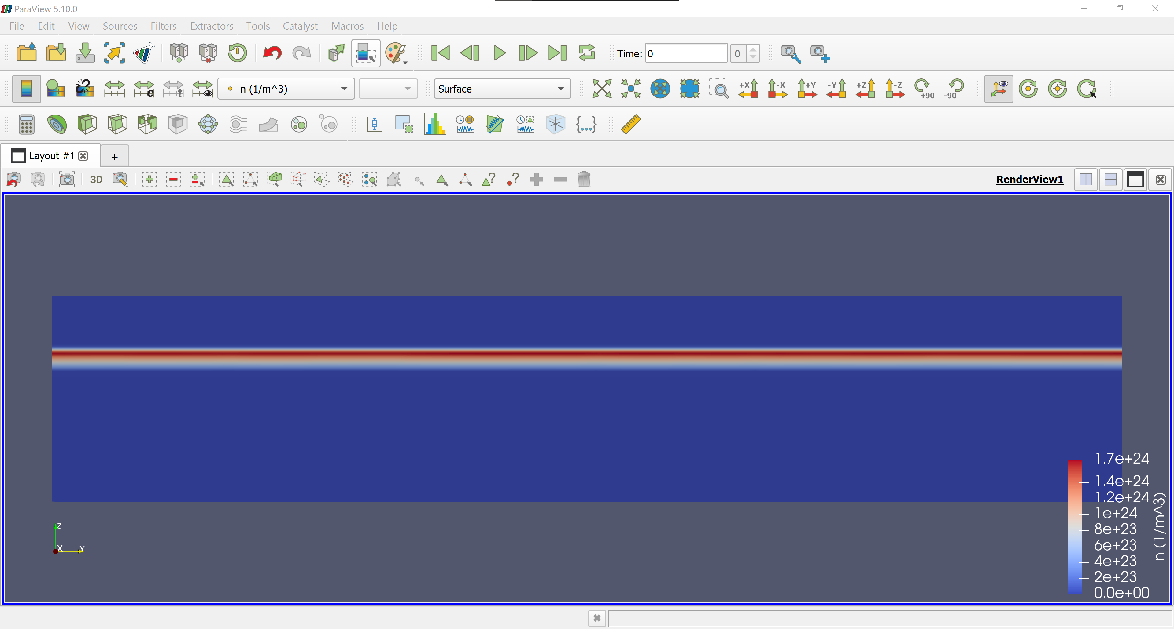
Fig. 3.4.3 Electron density
It may be observed that the 2DEG forming at the spacer–substrate interface spreads out along \(z\) much more than the equivalent results for the nonlinear Poisson solver; see Fig. 2.4.11. This is due to the uncertainty principle, which forces envelope functions in the quantum well and thus the electron density to have relatively large spreads along \(z\). This results in a distinct potential profile compared to what was obtained via the nonlinear Poisson solver. In the following section, we will see how this impacts the energy levels in the quantum dot.
3.5. Solving Schrödinger’s equation in the quantum dot
It remains to compute the eigenspectrum of the quantum dot, which we do following the method described in the previous tutorial.
# Get the potential energy from the band edge for usage in the Schrodinger
# solver
d.set_V_from_phi()

# Create a subdevice for the dot region
qd_subdevice = SubDevice(d, submesh_qd)

# Create a Schrodinger solver
schrod_solver = SchrodingerSolver(qd_subdevice)

# Solve Schrodinger's equation
schrod_solver.solve()

# Print energies
qd_subdevice.print_energies()
This results in the following eigenenergies:
Energy levels (eV)
[-0.00095922 0.00963754 0.01345700 0.02037420 0.02414355 0.02842833
  0.03171245 0.03506137 0.03929578 0.04272202]
It may be noticed that the ground state is slightly below the Fermi energy (\(0~\textrm{eV}\)). This is to be compared to the results of the previous tutorial based on the nonlinear Poisson solver, for which the ground state was slightly above the Fermi energy. This discrepancy may be expected to result in significant variations in, e.g., quantum dot occupation or qubit dynamics. In addition, tunneling rates between a source or drain in the 2DEG and the quantum dot may be substantially different when the quantum well solver is used to describe reservoirs (instead of the usual non-linear Poisson solver) because of different potential barrier heights. Likewise, the lever arm of the source or drain on the quantum dot may be affected by quantization of the reservoir charge carriers. These considerations may justify our use of the quantum-well solver, despite its higher computational cost than the nonlinear Poisson solver, in situations where such effects are of experimental relevance.
Finally, the ground state, 1st excited state, and 2nd excited states are saved
in a .vtu file.
In the next tutorials of the Practical Application, for computational simplicity, our simulations will be based on the nonlinear Poisson solver rather than the quantum-well solver.
# Save the first few eigenstates
outfile_eigenfunctions = str(script_dir / "output" / "eigenfunctions_qw.vtu")
out_dict = {"Ground": qd_subdevice.eigenfunctions[:,0],
    "1st excited": qd_subdevice.eigenfunctions[:,1],
    "2nd excited": qd_subdevice.eigenfunctions[:,2]}
io.save(outfile_eigenfunctions, out_dict, submesh_qd)
3.6. Full code
__copyright__ = "Copyright 2022-2025, Nanoacademic Technologies Inc."

from qtcad.device import constants as ct
from qtcad.device.mesh3d import Mesh, SubMesh
from qtcad.device import io
from qtcad.device import materials as mt
from qtcad.device import Device, SubDevice
from qtcad.device.quantum_well import Solver as QuantumWellSolver
from devicegen import DeviceGenerator
from qtcad.device.mesh2d import Mesh as Mesh2D
from qtcad.device.schrodinger import Solver as SchrodingerSolver
from qtcad.device.poisson import SolverParams as PoissonSolverParams
from qtcad.device.schrodinger import SolverParams as SchrodingerSolverParams
from qtcad.device.quantum_well import SolverParams as QuantumWellSolverParams
import pathlib

# Input file
script_dir = pathlib.Path(__file__).parent.resolve()
path_mesh = str(script_dir/'meshes'/'gated_dot.msh')

# Load the mesh
scaling = 1e-6
mesh = Mesh(scaling,path_mesh)
mesh.show()

# Create device
d = Device(mesh, conf_carriers="e")
d.set_temperature(0.1)

# Ionized dopant density
doping = 3e18*1e6   # In SI units

# Set up materials in heterostructure stack
d.new_region("cap", mt.GaAs)
d.new_region("barrier", mt.AlGaAs)
d.new_region("dopant_layer", mt.AlGaAs,ndoping=doping)
d.new_region("spacer_layer", mt.AlGaAs)
d.new_region("spacer_dot", mt.AlGaAs)
d.new_region("two_deg", mt.GaAs)
d.new_region("two_deg_dot", mt.GaAs)
d.new_region("substrate", mt.GaAs)
d.new_region("substrate_dot", mt.GaAs)

# Align the bands across hetero-interfaces using GaAs as the reference material
d.align_bands(mt.GaAs)

# Remove unphysical charge from cap and barrier
d.new_insulator("cap")
d.new_insulator("barrier")

# Applied potentials
Vtop_1 = -0.5
Vtop_2 = -0.5
Vtop_3 = -0.5
Vbottom_1 = -0.5
Vbottom_2 = -0.5
Vbottom_3 = -0.5

# Work function of the metallic gates at midgap of GaAs
barrier = 0.834*ct.e    # n-type Schottky barrier height

# Set up boundary conditions
d.new_schottky_bnd("top_gate_1", Vtop_1, barrier)
d.new_schottky_bnd("top_gate_2", Vtop_2, barrier)
d.new_schottky_bnd("top_gate_3", Vtop_3, barrier)
d.new_schottky_bnd("bottom_gate_1", Vbottom_1, barrier)
d.new_schottky_bnd("bottom_gate_2", Vbottom_2, barrier)
d.new_schottky_bnd("bottom_gate_3", Vbottom_3, barrier)
d.new_ohmic_bnd("ohmic_bnd")

# Create a submesh including only the dot region
submesh_qd = SubMesh(mesh, ["spacer_dot","two_deg_dot","substrate_dot"])
submesh_qd.show()

# Set up the dot region in which no charge is allowed in the quantum-well solver
d.set_dot_region(submesh_qd)

# Create subdevice for the quantum well region
submesh_qw = SubMesh(mesh, ["spacer_layer", "spacer_dot", "two_deg", "two_deg_dot", "substrate", "substrate_dot"])
submesh_qw.show()
qw_subdevice = SubDevice(d, submesh_qw)

# Solver parameters for the quantum-well solver
poisson_params = PoissonSolverParams()
schrod_params = SchrodingerSolverParams({"ti_directions": ["x", "y"]})
qw_params = QuantumWellSolverParams()
qw_params.poisson_solver_params = poisson_params
qw_params.schrod_solver_params = schrod_params

# define coordinates for linecuts through the quantum well using devicegen
char_len = 20 * 1e-3
path_layout = str(script_dir / "layouts" / "gated_qd.txt")
path_geo_2d = str(script_dir / "layouts" / "gated_qd_2d.geo")
dG = DeviceGenerator(path_layout, outfile=path_geo_2d, h=char_len)
path_mesh_2d = str(script_dir / "meshes" / "gated_qw_2d.msh")
dG.save_mesh(mesh_name=path_mesh_2d)
mesh_2d = Mesh2D(scaling, path_mesh_2d)
mesh_2d.show()

# Set up quantum-well solver
qw_solver = QuantumWellSolver(
    d=d, qw_subdevice=qw_subdevice, coords=mesh_2d, solver_params=qw_params
    )

# Solve
qw_solver.solve()

# Save the conduction band edge in .vtu format
outfile_cond_band_edge = str(script_dir / "output" / "cond_band_edge_qw.vtu")
out_dict = {"EC (eV)": d.cond_band_edge()/ct.e}
io.save(outfile_cond_band_edge, out_dict, mesh)

# Save the electron density in .vtu format
outfile_electron_dens = str(script_dir / "output" / "electron_dens_qw.vtu")
out_dict = {"n (1/m^3)": d.n}
io.save(outfile_electron_dens, out_dict, mesh)

# Get the potential energy from the band edge for usage in the Schrodinger
# solver
d.set_V_from_phi()

# Create a subdevice for the dot region
qd_subdevice = SubDevice(d, submesh_qd)

# Create a Schrodinger solver
schrod_solver = SchrodingerSolver(qd_subdevice)

# Solve Schrodinger's equation
schrod_solver.solve()

# Print energies
qd_subdevice.print_energies()

# Save the first few eigenstates
outfile_eigenfunctions = str(script_dir / "output" / "eigenfunctions_qw.vtu")
out_dict = {"Ground": qd_subdevice.eigenfunctions[:,0],
    "1st excited": qd_subdevice.eigenfunctions[:,1],
    "2nd excited": qd_subdevice.eigenfunctions[:,2]}
io.save(outfile_eigenfunctions, out_dict, submesh_qd)