4. Calculating the lever arm of a quantum dot
4.1. Requirements
4.1.1. Software components
QTCAD
4.1.2. Mesh file
qtcad/examples/practical_application/meshes/gated_dot.msh
4.1.3. Python script
qtcad/examples/practical_application/4-lever_arm.py
4.1.4. References
4.2. Briefing
In the second tutorial (Simulating bound states in a quantum dot using the Poisson and Schrödinger solvers), we have used QTCAD to compute, among other things, the discrete energy levels inside the quantum dot for one configuration of external voltages. Specifically, all six gate voltages were fixed to \(-0.5\textrm{ V}\). These gates create the confinement potential for electrons in the quantum dot. In particular, they control the depth of this potential, and therefore the energy levels in the dot. In this tutorial, we will explore the dependence of these energy levels on the external voltages. In particular, we will extract the lever arm, a unitless parameter which describes the strength of the capacitive coupling between the gate and the dot. For perfect capacitive coupling, the lever arm is equal to \(1\), which means that a change of \(1 \textrm{ V}\) in gate voltage results in a change in \(1 \textrm{ eV}\) in the energy levels. More realistically, the lever arm is between \(0\) and \(1\). See Lever arm theory for a more in-depth discussion of lever arms from a theoretical perspective.
4.3. Setting up the device
4.3.1. Header
We start by importing relevant modules.
from qtcad.device import constants as ct
from qtcad.device.mesh3d import Mesh
from qtcad.device import materials as mt
from qtcad.device import Device
from qtcad.device.poisson import SolverParams as PoissonSolverParams
from qtcad.device.leverarm import Solver as LeverArmSolver
from qtcad.device.leverarm import SolverParams as LeverArmSolverParams
import pathlib
import numpy as np
import matplotlib.pyplot as plt
import pickle
These modules are the same as in Simulating bound states in a quantum dot using the Poisson and Schrödinger solvers with
the addition of the numpy modules for arrays and numerical computing
tools, the matplotlib module for data visualization, and the
pickle module for object serialization. In addition, we now import
the Solver from the
leverarm module, along with non-linear
Poisson SolverParams
and lever-arm SolverParams
classes that will be used to configure the solvers.
4.3.2. Defining the device
As was done in the second tutorial, we load the device mesh, define the device’s material composition, define the external gate voltages, and set the appropriate boundary conditions.
# Input file
script_dir = pathlib.Path(__file__).parent.resolve()
path_mesh = str(script_dir/'meshes'/'gated_dot.msh')
path_out = script_dir / 'output' / 'electric_potential'

# Applied potentials
Vtop_1 = -0.5
Vtop_2 = -0.5
Vtop_3 = -0.5
Vbottom_1 = -0.5
Vbottom_2 = -0.5
Vbottom_3 = -0.5

# Work function of the metallic gates at midgap of GaAs
barrier = 0.834*ct.e    # n-type Schottky barrier height

# Ionized dopant density
doping = 3e18*1e6   # In SI units

# Load the mesh
scaling = 1e-6
mesh = Mesh(scaling,path_mesh)

# Create device
d = Device(mesh, conf_carriers="e")
d.set_temperature(0.1)

# Set up materials in heterostructure stack
d.new_region("cap", mt.GaAs)
d.new_region("barrier", mt.AlGaAs)
d.new_region("dopant_layer", mt.AlGaAs,ndoping=doping)
d.new_region("spacer_layer", mt.AlGaAs)
d.new_region("spacer_dot", mt.AlGaAs)
d.new_region("two_deg", mt.GaAs)
d.new_region("two_deg_dot", mt.GaAs)
d.new_region("substrate", mt.GaAs)
d.new_region("substrate_dot", mt.GaAs)

# Align the bands across hetero-interfaces from atomistic data
# using GaAs as the reference material
d.align_bands(mt.GaAs)

# Remove unphysical charge from cap and barrier
d.new_insulator("cap")
d.new_insulator("barrier")

# Set up boundary conditions
d.new_schottky_bnd("top_gate_1", Vtop_1, barrier)
d.new_schottky_bnd("top_gate_2", Vtop_2, barrier)
d.new_schottky_bnd("top_gate_3", Vtop_3, barrier)
d.new_schottky_bnd("bottom_gate_1", Vbottom_1, barrier)
d.new_schottky_bnd("bottom_gate_2", Vbottom_2, barrier)
d.new_schottky_bnd("bottom_gate_3", Vbottom_3, barrier)
d.new_ohmic_bnd("ohmic_bnd")
We then define and set the dot region, thus specifying that the device contains a quantum dot.
# Create a list for the dot region
dot_region = ["spacer_dot","two_deg_dot","substrate_dot"]

# Set up the dot region in which no classical charge is allowed
d.set_dot_region(dot_region)
Finally, we set up the parameters of the Poisson solver that will be used
by the lever arm calculator in the same way as in the second tutorial, i.e.,
by instantiating a Poisson
SolverParams object. We then
instantiate a lever-arm
SolverParams object, in which
we input the Poisson
SolverParams object defined first
to configure the electrostatics solver that underpins the lever-arm
calculation.
# Create the parameters of the non-linear Poisson solver
poisson_solver_params = PoissonSolverParams({"tol": 1e-3, "maxiter": 100})

# Create the parameters of the lever-arm solver
lever_arm_solver_params = LeverArmSolverParams({
    "pot_solver_params": poisson_solver_params
})
4.4. Sweeping over the plunger gate potential
At this point, all simulation parameters have been specified. Since our goal is to study the lever arm, we should perform a gate potential sweep. As we may recall from From photomask to mesh generation, the quantum dot is surrounded by six gates as illustrated below.
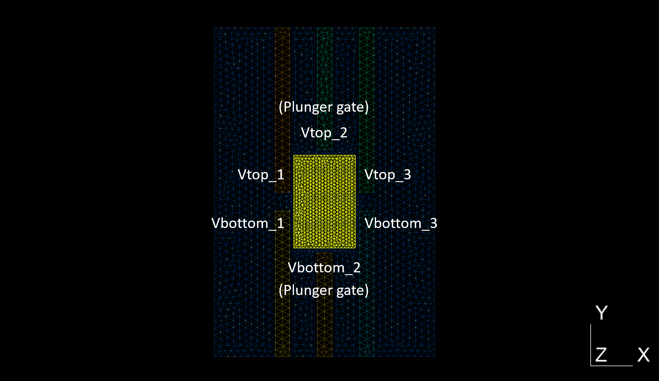
Fig. 4.4.3 Gates surrounding the quantum dot
Potentials can be applied independently on each gate: these correspond to the
parameters Vtop_1, V_bottom_1, V_top_2, V_bottom_2,
Vtop_3, and V_bottom_3 that were previously set to -0.5. In the
following, we will repeatedly solve both Poisson and Schrödinger equations
in the quantum dot, keeping Vtop_1, V_bottom_1, Vtop_3, and
V_bottom_3 fixed at -0.5 and sweeping V_top_2, V_bottom_2
from -1.0 to 0.0. Collectively, the two middle-column gates labeled by
the index 2 are called “plunger gates.”
We create the lever arm solver and calculate the lever arm with
# Create and run the lever arm solver
print("Getting lever arm data for top_gate_2, bottom_gate_2")
Vp_vals = np.linspace(-1.0, 0.0, 11)
lever_arm_slv = LeverArmSolver(d, ["top_gate_2", "bottom_gate_2"], Vp_vals,
    dot_region=dot_region, solver_params=lever_arm_solver_params,
    out_path=path_out)
poly_coeffs = lever_arm_slv.solve()
Here, Vp_vals is an array containing the plunger gate potential
values over which we will solve Schrödinger’s equation.
After defining this voltage sweep, we instantiate the lever arm
Solver
with the following arguments:
The device over which Poisson’s equation is solved.
The list of boundaries at which the gate potential is applied.
The gate potential values.
The list of regions defining the submesh over which Schrödinger’s equation is solved for each applied potential (dot region).
The parameters to use for the lever-arm solver.
The path to the output files in which the electric potential will be saved.
In addition, parameters for the Schrödinger solver may be specified
(see the lever-arm SolverParams
class API reference). Here we use the default values.
Upon instantiation, the lever arm solver launches a loop that sweeps over
applied biases. For each bias, the non-linear Poisson and single-body
Schrödinger’s equations are successively solved. The eigenenergies for each
gate configuration are stored in the
energies
attribute of the lever arm
Solver
object.
Finally, after instantiation, the
solve
method of the
Solver
object may be used to produce a linear fit of the ground state energy as a
function of gate bias. The first-order coefficient of this linear fit gives
the lever arm, i.e., the slope of the ground state energy as a function of
plunger gate bias in our example.
For our quantum dot, we may print the lever arm with
print(f"The lever arm is {np.abs(poly_coeffs[0])/ct.e}")
which yields the following.
The lever arm is 0.07110731522471611
Namely, typically, for every increment in \(1\textrm{ V}\) in the plunger gate potential, the ground state eigenenergy decreases by approximately \(71.4~\textrm{meV}\). Note that, above, we take the absolute value since the lever arm is always defined as strictly positive.
Next, the results, i.e. the eigenenergies as a function of the plunger gate potential, are plotted.
# Plot results
fig, ax1 = plt.subplots()

ax1.set_ylabel("Energy (eV)")
ax1.set_xlabel("Plunger gate voltage (V)")
for i, data in enumerate(lever_arm_slv.energies.T/ct.e):
    ax1.plot(Vp_vals, data, label=f"state {i}")

fig.set_size_inches(7,5)
fig.set_dpi(100)
plt.legend()
plt.show()
This results in the following figure.
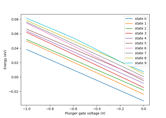
Fig. 4.4.4 Lever arm in a quantum dot
The results can then be saved, here using the pickle module.
# Pickle results
path_pkl = str(script_dir/'output'/'lever_arm.pkl')
outfile = open(path_pkl, 'wb')
pickle.dump((Vp_vals, lever_arm_slv.energies.T/ct.e), outfile)
4.5. Full code
__copyright__ = "Copyright 2022-2025, Nanoacademic Technologies Inc."

from qtcad.device import constants as ct
from qtcad.device.mesh3d import Mesh
from qtcad.device import materials as mt
from qtcad.device import Device
from qtcad.device.poisson import SolverParams as PoissonSolverParams
from qtcad.device.leverarm import Solver as LeverArmSolver
from qtcad.device.leverarm import SolverParams as LeverArmSolverParams
import pathlib
import numpy as np
import matplotlib.pyplot as plt
import pickle

# Input file
script_dir = pathlib.Path(__file__).parent.resolve()
path_mesh = str(script_dir/'meshes'/'gated_dot.msh')
path_out = script_dir / 'output' / 'electric_potential'

# Applied potentials
Vtop_1 = -0.5
Vtop_2 = -0.5
Vtop_3 = -0.5
Vbottom_1 = -0.5
Vbottom_2 = -0.5
Vbottom_3 = -0.5

# Work function of the metallic gates at midgap of GaAs
barrier = 0.834*ct.e    # n-type Schottky barrier height

# Ionized dopant density
doping = 3e18*1e6   # In SI units

# Load the mesh
scaling = 1e-6
mesh = Mesh(scaling,path_mesh)

# Create device
d = Device(mesh, conf_carriers="e")
d.set_temperature(0.1)

# Set up materials in heterostructure stack
d.new_region("cap", mt.GaAs)
d.new_region("barrier", mt.AlGaAs)
d.new_region("dopant_layer", mt.AlGaAs,ndoping=doping)
d.new_region("spacer_layer", mt.AlGaAs)
d.new_region("spacer_dot", mt.AlGaAs)
d.new_region("two_deg", mt.GaAs)
d.new_region("two_deg_dot", mt.GaAs)
d.new_region("substrate", mt.GaAs)
d.new_region("substrate_dot", mt.GaAs)

# Align the bands across hetero-interfaces from atomistic data
# using GaAs as the reference material
d.align_bands(mt.GaAs)

# Remove unphysical charge from cap and barrier
d.new_insulator("cap")
d.new_insulator("barrier")

# Set up boundary conditions
d.new_schottky_bnd("top_gate_1", Vtop_1, barrier)
d.new_schottky_bnd("top_gate_2", Vtop_2, barrier)
d.new_schottky_bnd("top_gate_3", Vtop_3, barrier)
d.new_schottky_bnd("bottom_gate_1", Vbottom_1, barrier)
d.new_schottky_bnd("bottom_gate_2", Vbottom_2, barrier)
d.new_schottky_bnd("bottom_gate_3", Vbottom_3, barrier)
d.new_ohmic_bnd("ohmic_bnd")

# Create a list for the dot region
dot_region = ["spacer_dot","two_deg_dot","substrate_dot"]

# Set up the dot region in which no classical charge is allowed
d.set_dot_region(dot_region)

# Create the parameters of the non-linear Poisson solver
poisson_solver_params = PoissonSolverParams({"tol": 1e-3, "maxiter": 100})

# Create the parameters of the lever-arm solver
lever_arm_solver_params = LeverArmSolverParams({
    "pot_solver_params": poisson_solver_params
})

# Create and run the lever arm solver
print("Getting lever arm data for top_gate_2, bottom_gate_2")
Vp_vals = np.linspace(-1.0, 0.0, 11)
lever_arm_slv = LeverArmSolver(d, ["top_gate_2", "bottom_gate_2"], Vp_vals,
    dot_region=dot_region, solver_params=lever_arm_solver_params,
    out_path=path_out)
poly_coeffs = lever_arm_slv.solve()

print(f"The lever arm is {np.abs(poly_coeffs[0])/ct.e}")

# Plot results
fig, ax1 = plt.subplots()

ax1.set_ylabel("Energy (eV)")
ax1.set_xlabel("Plunger gate voltage (V)")
for i, data in enumerate(lever_arm_slv.energies.T/ct.e):
    ax1.plot(Vp_vals, data, label=f"state {i}")

fig.set_size_inches(7,5)
fig.set_dpi(100)
plt.legend()
plt.show()

# Pickle results
path_pkl = str(script_dir/'output'/'lever_arm.pkl')
outfile = open(path_pkl, 'wb')
pickle.dump((Vp_vals, lever_arm_slv.energies.T/ct.e), outfile)