7. Electric dipole spin resonance and Rabi oscillations
7.1. Requirements
7.1.1. Software components
QTCAD
7.1.2. Mesh file
qtcad/examples/practical_application/meshes/gated_dot.msh
7.1.3. Python script
qtcad/examples/practical_application/7-EDSR.py
7.1.4. References
7.2. Briefing
In the previous tutorial, we obtained the charge-stability diagram of our gated quantum dot. Using this diagram, we can extract the voltage configurations under which a single electron resides in the quantum dot. Furthermore, we have computed the energy levels of such an electron. Assuming that the second-excited eigenenergy is sufficiently far from the first-excited eigenenergy, our quantum dot’s electron constitutes a qubit. Typically, for a single quantum dot used as a Loss-DiVincenzo spin qubit, the first two levels correspond to an electron in its orbital ground state with Zeeman-split spin states, while the second and third excited states contain an excitation of the electron’s orbital degree of freedom. In this tutorial, we will simulate an electric dipole spin resonance (EDSR) experiment on this qubit, driving transitions between the ground state and first-excited state using a time-varying voltage applied to a gate and an inhomogeneous magnetic field.
7.3. Setting up the device
7.3.1. Header
We start by importing relevant modules.
import numpy as np
import pathlib
from matplotlib import pyplot as plt
import qutip
import pickle

from qtcad.device import constants as ct
from qtcad.device.mesh3d import Mesh, SubMesh
from qtcad.device import io

from qtcad.device import Device, SubDevice
from qtcad.device.schrodinger import Solver, SolverParams
from qtcad.device import materials as mt

from qtcad.device.operators import Zeeman, Gate
from qtcad.qubit import dynamics
We have previously seen all of these modules, except for the operators
and dynamics modules.
The former is used to simulate EDSR experiments—specifically to modulate the
voltages applied to the gates of quantum dots and compute the
resulting potential energy matrices.
The latter contains various calculators and visualizers for system dynamics,
and harnesses the QuTiP python library.
7.3.2. Creating a quantum dot with a single electron
The next step is to define our device and set external voltages, as was done in
previous tutorials.
Based on the charge-stability diagram obtained in Calculating the charge-stability diagram of a quantum dot, a
plunger gate potential of \(-0.4\textrm{ V}\) results in a single electron
residing in the dot.
Thus, the applied potentials are defined to reflect this voltage configuration;
notably Vtop_2 and Vbottom_2 are set to -0.4.
Furthermore, the electric potential, d.phi, is loaded from the file
electric_potential_-0.400V.hdf5
(recall that using the
set_potential method of the
Device class ensures that the device’s
confinement potential energy is updated accordingly).
# Load the mesh
script_dir = pathlib.Path(__file__).parent.resolve()
path_mesh = str(script_dir /'meshes'/'gated_dot.msh')
scaling = 1e-6
mesh = Mesh(scaling, path_mesh)

# Create device
d = Device(mesh, conf_carriers="e")
d.set_temperature(0.1)

# Number of orbital states to consider in Schrodinger solver
num_states = 3

# # Applied potentials
Vtop_1 = -0.5
Vtop_2 = -0.4
Vtop_3 = -0.5
Vbottom_1 = -0.5
Vbottom_2 = -0.4
Vbottom_3 = -0.5

# Work function of the metallic gates at midgap of GaAs
barrier = 0.834*ct.e    # n-type Schottky barrier height

# Ionized dopant density
doping = 3e18*1e6   # In SI units

# Set up materials in heterostructure stack
d.new_region("cap", mt.GaAs)
d.new_region("barrier", mt.AlGaAs)
d.new_region("dopant_layer", mt.AlGaAs,ndoping=doping)
d.new_region("spacer_layer", mt.AlGaAs)
d.new_region("spacer_dot", mt.AlGaAs)
d.new_region("two_deg", mt.GaAs)
d.new_region("two_deg_dot", mt.GaAs)
d.new_region("substrate", mt.GaAs)
d.new_region("substrate_dot", mt.GaAs)

# Remove unphysical charge from cap and barrier
d.new_insulator("cap")
d.new_insulator("barrier")

# Align the bands across hetero-interfaces using GaAs as the reference material
d.align_bands(mt.GaAs)

# Set up boundary conditions
d.new_schottky_bnd("top_gate_1", Vtop_1, barrier)
d.new_schottky_bnd("top_gate_2", Vtop_2, barrier)
d.new_schottky_bnd("top_gate_3", Vtop_3, barrier)
d.new_schottky_bnd("bottom_gate_1", Vbottom_1, barrier)
d.new_schottky_bnd("bottom_gate_2", Vbottom_2, barrier)
d.new_schottky_bnd("bottom_gate_3", Vbottom_3, barrier)
d.new_ohmic_bnd("ohmic_bnd")

# Load the confinement potential from previous run
path_in = str(script_dir/"output"/"electric_potential_-0.400V.hdf5")
d.set_potential(io.load(path_in))

# Create a submesh in which to solve Schrodinger's equation
submesh = SubMesh(mesh, ["spacer_dot", "two_deg_dot", "substrate_dot"])
subdevice = SubDevice(d,submesh)
7.3.3. Solving Schrödinger’s equation
Following the same method as in the previous tutorials, we now solve the
Schrödinger equation within the subdevice representing the quantum dot.
# Solve Schrodinger's equation for single electrons
params = SolverParams()
params.num_states = num_states
params.tol = 1e-9   # Decrease tolerance to stabilize Rabi frequency
s = Solver(subdevice, solver_params=params)
s.solve()

# # Plot eigenstates
# subdevice.print_energies()
# from device import analysis as an
# an.plot_slices(submesh, np.absolute(subdevice.eigenfunctions[:,0])**2,
#     z=-42e-9)
# an.plot_slices(submesh, np.absolute(subdevice.eigenfunctions[:,1])**2,
#     z=-42e-9)
# an.plot_slices(submesh, np.absolute(subdevice.eigenfunctions[:,2])**2,
#     z=-42e-9)
The eigenenergies and eigenfunctions may be shown using the commented code.
7.4. Adding perturbations
7.4.1. Setting up the magnetic fields
The EDSR experiment we wish to simulate uses (1) a homogeneous magnetic field
aligned with the \(y\) axis, and (2) a weaker inhomogeneous
magnetic-field component aligned in the \(z\) direction, whose strength
varies linearly as a function of \(y\).
This second magnetic-field component may be produced by a micromagnet, and is
typically called a slanting field in the EDSR literature.
Such a slanting field implements an effective spin–orbit coupling for the
electron confined to our quantum dot [see Eq. (12.1) in
the Quantum control theory section].
The total magnetic field is defined by a function over the coordinates,
\(x\), \(y\), and \(z\).
This function is given by B_field below.
# Set magnetic field
def B_field(x, y, z):
   B0 = 0.6 # Homogeneous B field
   # Position-dependent B - due to micromagnet
   b = 0.3/1e-6 # 0.3 T/micron

   return np.array([0, B0, b*y])
We can now investigate the influence of the magnetic field via the Zeeman
effect on the quantum-dot eigenstates.
The subdevice and the magnetic field, B_field are passed to a
Zeeman operator, whose
solve method computes matrix
elements of the Zeeman Hamiltonian within the subspace spanned by the
subdevice eigenstates (subdevice.eigenfunctions).
Z = Zeeman(subdevice, B = B_field)
Z.solve()

# The (undriven) system Hamiltonian will include the Zeeman interaction.
H0Z = np.diag(Z.energies - Z.energies[0])
This method then diagonalizes the Hamiltonian \(H_0 + H_Z\) within this
subspace, where \(H_0\) is the unperturbed Hamiltonian (associated with the
Schrödinger solver, s above) and \(H_Z\) is the Zeeman Hamiltonian.
The eigenenergies of \(H_0 + H_Z\) are stored in Z.energies and the
eigenfunctions are stored in Z.eigenfunctions.
The undriven system Hamiltonian, \(\hat{H}_0 + \hat{H}_Z\), in its
eigenbasis is stored in the variable H0Z.
7.4.2. The potential energy matrix
Having accounted for the Zeeman effect via the
Z object, we define a
Gate operator
which computes matrix elements related to the drive of the system (which is
applied through time-dependent voltages applied to gates).
The operators module is written in such a
way that an operator can be passed to another operator.
In this specific case, we will pass a
Zeeman operator, Z, to a
Gate operator, G.
num_V = 6
gate_biases = np.linspace(-0.5, -0.4, num=num_V)
U_shape = (num_V, len(Z.energies), len(Z.energies))
U = np.zeros(U_shape, dtype=complex)
for i, V in enumerate(gate_biases):
   G = Gate(Z, 'top_gate_3', V, phys_d=d, NL=False, base_bias=-0.5)
   U[i, :, :] = G.get_operator_matrix()
Here we loop over different gate biases, gate_biases.
This variable is an array containing the biases we wish to apply to a gate.
For each bias, V, we create a
Gate operator, G.
The first argument of the Gate constructor is the object containing the
information about the unperturbed system (unperturbed energies and
eigenfunctions), in this case, Z.
The second input is a string labelling the boundary for which we wish to modify
the applied bias, 'top_gate_3', and the third input is the bias we wish to
apple, V.
We must specify that 'top_gate_3' is a boundary of the full device, d,
by passing d as a keyword argument (phys_d).
Finally, for this specific example we set NL=False indicating that we will
solve for the potential energy (perturbation) due to this change in bias on
'top_gate_3' using a linear Poisson solver instead of a non-linear Poisson
solver.
In essence, this is equivalent to neglecting the redistribution of classical
charge caused by the perturbation.
Finally, we use the base_bias keyword argument to specify that the default
configuration of the device is one where the bias applied to 'top_gate_3'
is \(-0.5\textrm{ V}\) (see Gate Operator for more details).
We then use the
get_operator_matrix method to
compute the matrix elements of the potential-energy perturbation in the
eigenbasis of Z.
For additional details on the EDSR procedure implemented in QTCAD, see the Time-dependent Hamiltonian subsection of the Quantum control theory section.
After the loop is complete, we are left with H0Z, a 2D array containing the
undriven Hamiltonian in its eigenbasis and shifted so that the ground state has
an energy of \(0\) and U a 3D array containing the drive operator in
the same basis as H0Z for each element in gate_biases.
We can then plot the matrix elements of the perturbation as a function of
gate_biases.
In this specific case, we plot U[:, 0, 1] (the first set of indices, :,
runs over the elements of gate_biases).
Each matrix U[i,:,:] corresponds to the confinement potential
perturbation \(\delta \hat V\) introduced in
Eq. (12.4) of the
Quantum control theory section, projected in the basis of the two
lowest-energy eigenstates of the Zeeman Hamiltonian, and for the
\(i\)-th applied gate bias.
# The potential energy matrix is a linear function of the applied voltage
fig= plt.figure()

# Plot - 01 matrix element
ax1 = fig.add_subplot(111)
ax1.plot(gate_biases, np.real(U[:, 0, 1])/ct.e, '.-', label="Real")
ax1.plot(gate_biases, np.imag(U[:, 0, 1])/ct.e, '.-', label="Imaginary")
ax1.set_xlabel(r'$\varphi^\mathrm{bias}$', fontsize=20)
ax1.set_ylabel(r'$\delta V_{01}(\varphi^\mathrm{bias})$ (eV)', fontsize=20)
ax1.grid()
ax1.legend()
fig.tight_layout()
plt.show()
This results in the figure below, which clearly shows that this matrix element
is a linear function of the applied voltage. It can similarly be verified that
all other elements of U are linear functions of the applied voltage.
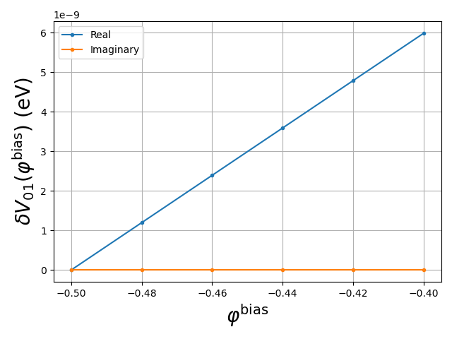
Fig. 7.4.4 The elements of the confinement potential perturbation matrix \(\delta \hat V\) are linear functions of the applied voltage
This linearity will greatly simplify our simulations of the dynamics of our spin qubit under a time-varying electric field: we can simply use a linear interpolation of the confinement potential perturbation matrix \(\delta \hat V\) to model the potential energy matrices for an arbitrary applied voltage.
In preparation of dynamics simulations, we define delta_V as the element
of U corresponding to the largest voltage in gate_biases, and shift
its diagonal so as to ensure that delta_V[0,0] is 0. This arbitrary
potential-energy shift does not influence the physical solution but will later
eliminate fast oscillating terms proportional to the identity matrix that
would otherwise slow down the solution of the time-dependent Schrödinger
equation.
# Use the fact that the perturbing potential is a linear function of the
# applied voltage.
delta_V = U[-1]
# Reset the zero of energy (ground state has E!=0).
np.fill_diagonal(delta_V, delta_V.diagonal()-delta_V[0,0])
We can also print the unperturbed system eigenenergies.
# System Hamiltonian in the eigenbasis is diagonal
print(f'evals (eV):{(np.diagonal(H0Z) - H0Z[0,0])/ct.e}')
This results in the following.
evals (eV):[0.00000000e+00 1.46160020e-05 1.03161274e-02 1.03307082e-02
 1.45791459e-02 1.45937110e-02]
It can be noticed that the ground state and first-excited state are separated by merely \(15~\mu\textrm{eV}\) while the first-excited state and second-excited state are separated by a quantity three orders of magnitude greater. The spectrum is thus compatible with a well-behaved spin qubit. A good approximation to model the dynamics of our spin qubit is thus a projection onto these two states, ignoring higher-energy states.
7.5. EDSR—Projection on the 2-level subspace
To model the dynamics of such a two-level system, we use the Dynamics class.
# Simple EDSR calculation. The calculation is performed by projecting onto
# the relevant 2 dimensional subspace. Here we are studying transitions
# between the ground state and the first excited state. The optional
# parameter plot is set to true to visualize the results.
dyn = dynamics.Dynamics()
This class has a method, transition_2_levels, which projects the system
Hamiltonian and the drive Hamiltonian onto the appropriate two-level subspace
and compute its dynamics.
The transition_2_levels() method implements the theory described in the
subsection called A simple scenario: a driven two-level system under the rotating-wave approximation in the Quantum control theory section.
result, h0, u, omega0, omega_rabi = dyn.transition_2_levels(1, 0, H0Z,
   delta_V, plot=True, npts=20000)

# Save the projections of H0 and delta_V on the 2-dimensional subspace
# for later use
np.save(str(script_dir/'output'/'h0.npy'), h0)
np.save(str(script_dir/'output'/'u.npy'), u)
The system and drive Hamiltonians are specified as H0 and delta_V,
respectively. The indices describing our two-level subspace are given as the
first two arguments of transition_2_levels: 1 is the state labeled as
\(\ket{\uparrow}\) and 0 is the state labeled as \(\ket{\downarrow}\),
the latter of which is taken as the initial state in the simulation. The
method transition_2_levels returns a number of variables: result is a
QuTiP object containing information about the dynamics, h0 is the system
Hamiltonian projected onto the two-level subspace, u is the drive
Hamiltonian projected onto the two-level subspace, omega0 is the resonance
frequency, and omega_rabi is the Rabi frequency of the transition between
the two states.
We also save h0 and u to files for later use (see Charge noise in quantum dots).
Furthermore, since we have specified plot=True,
transition_2_levels produces the following figure.
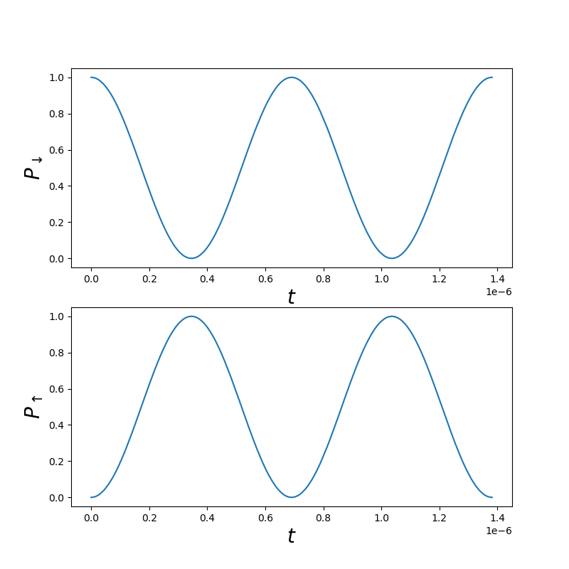
Fig. 7.5.10 Rabi oscillations for our qubit driven by EDSR in the two-level subspace approximation
7.6. EDSR—Beyond the 2-level subspace approximation
We now use QuTiP to go beyond the 2-level subspace and rotating-wave approximations of the previous section. We start by defining the various variables which will be used in the QuTiP simulation.
First, QuTiP assumes units in which \(\hbar=1\). We therefore adjust H0
and delta_V accordingly, converting them to QuTiP Qobj objects.
############################################################################

# More accurate but longer calculation beyond the projection into the 2-level
# subspace.

H0Z = qutip.Qobj(H0Z/ct.hbar) # system Hamiltonian in units of hbar
delta_V = qutip.Qobj(delta_V/ct.hbar) # potential energy matrix amplitude in units of hbar
To define our full Hamiltonian, H, as H0 plus a sinusoidal perturbation with
amplitude delta_V, we define the following.
H = [H0Z, [delta_V, 'cos(omega*t)']] # Full Hamiltonian - sinusoidal modulation of delta_V
Above, omega remains unspecified. We address this issue with the following.
# Drive the voltage at the resonance frequency of the transition we wish to
# observe
args = {'omega': omega0}
Next, we initialize the system in the ground state as follows.
# Initialize the system in its ground state
# The basis has 2*num_states; num_states orbital states and 2 spin states
psi0 = qutip.basis(2*num_states, 0) # initialize in the ground state
Having specified our Hamiltonian and initial state, we are ready to simulate
dynamics using the QuTiP mesolve function over a given list of times, which
we call t_list.
# Use the mesolve function of QuTiP to solve for the dynamics of the 6-level
# system.
T_Rabi = 2* np.pi / omega_rabi # Rabi cycle in the two-level limit
# array of times for which the solver should store the state vector
tlist = np.linspace(0, 2*T_Rabi, 300000)
result = qutip.mesolve(H, psi0, tlist, [], [], args=args, progress_bar=True)
This may take several minutes.
It remains to save and plot the results, which we do as follows.
# Plot the results with matplotlib and save them
# using the EDSR module to get projectors onto the 6 basis states
Proj = dyn.projectors(2*num_states)
population_data = []
outfile = open(str(script_dir/'output'/'EDSR.pkl'), 'wb')
# Plot projections onto each state.
fig, axes = plt.subplots(2,num_states)
for i in range(2):
   population_data_spin = []
   for j in range(num_states):
      expect = qutip.expect(Proj[num_states*i+j],result.states)
      population_data_spin += [expect]
      axes[i,j].plot(tlist, expect)
      axes[i,j].set_xlabel(r'$t$', fontsize=20)
      axes[i,j].set_ylabel(f'$P_{num_states*i+j}$', fontsize=20)
   population_data += [population_data_spin]
pickle.dump((tlist,population_data), outfile)
fig.tight_layout()
plt.show()
This results in the following figure.
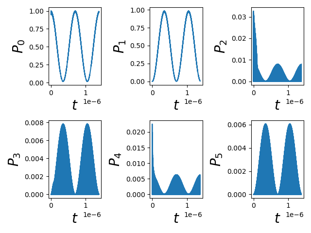
Fig. 7.6.6 Rabi oscillations for a spin qubit driven by EDSR beyond the two-level subspace approximation
We remark that while most of the population is exchanged between the two qubit states (\(0\) and \(1\)), some significant leakage into higher (non-computational) levels exists for the current drive amplitude and shape. This issue can typically be resolved using pulse shaping, for example so-called DRAG pulses. In addition, going beyond the rotating-wave oscillations, we see that the dynamics contains significant fast oscillatory components in addition to the ideal two-level Rabi oscillations considered above.
Warning
Because of the extreme difference in timescales between leakage dynamics
(which evolves over nanoseconds or less) and Rabi oscillations (which
occur over hundreds of nanoseconds or over microseconds), in a given
simulation, an exhaustive convergence analysis with respect to the
QuTiP time resolution and solver tolerance
(controlled by the atol, rtol, and nsteps solver
Options)
may be necessary.
Unless this convergence is
achieved, leakage oscillations may vary significantly between
machines and operating systems.
7.7. Full code
__copyright__ = "Copyright 2022-2025, Nanoacademic Technologies Inc."

import numpy as np
import pathlib
from matplotlib import pyplot as plt
import qutip
import pickle
from qtcad.device import constants as ct
from qtcad.device.mesh3d import Mesh, SubMesh
from qtcad.device import io
from qtcad.device import Device, SubDevice
from qtcad.device.schrodinger import Solver, SolverParams
from qtcad.device import materials as mt
from qtcad.device.operators import Zeeman, Gate
from qtcad.qubit import dynamics

# Load the mesh
script_dir = pathlib.Path(__file__).parent.resolve()
path_mesh = str(script_dir /'meshes'/'gated_dot.msh')
scaling = 1e-6
mesh = Mesh(scaling, path_mesh)

# Create device
d = Device(mesh, conf_carriers="e")
d.set_temperature(0.1)

# Number of orbital states to consider in Schrodinger solver
num_states = 3

# # Applied potentials
Vtop_1 = -0.5
Vtop_2 = -0.4
Vtop_3 = -0.5
Vbottom_1 = -0.5
Vbottom_2 = -0.4
Vbottom_3 = -0.5

# Work function of the metallic gates at midgap of GaAs
barrier = 0.834*ct.e    # n-type Schottky barrier height

# Ionized dopant density
doping = 3e18*1e6   # In SI units

# Set up materials in heterostructure stack
d.new_region("cap", mt.GaAs)
d.new_region("barrier", mt.AlGaAs)
d.new_region("dopant_layer", mt.AlGaAs,ndoping=doping)
d.new_region("spacer_layer", mt.AlGaAs)
d.new_region("spacer_dot", mt.AlGaAs)
d.new_region("two_deg", mt.GaAs)
d.new_region("two_deg_dot", mt.GaAs)
d.new_region("substrate", mt.GaAs)
d.new_region("substrate_dot", mt.GaAs)

# Remove unphysical charge from cap and barrier
d.new_insulator("cap")
d.new_insulator("barrier")

# Align the bands across hetero-interfaces using GaAs as the reference material
d.align_bands(mt.GaAs)

# Set up boundary conditions
d.new_schottky_bnd("top_gate_1", Vtop_1, barrier)
d.new_schottky_bnd("top_gate_2", Vtop_2, barrier)
d.new_schottky_bnd("top_gate_3", Vtop_3, barrier)
d.new_schottky_bnd("bottom_gate_1", Vbottom_1, barrier)
d.new_schottky_bnd("bottom_gate_2", Vbottom_2, barrier)
d.new_schottky_bnd("bottom_gate_3", Vbottom_3, barrier)
d.new_ohmic_bnd("ohmic_bnd")

# Load the confinement potential from previous run
path_in = str(script_dir/"output"/"electric_potential_-0.400V.hdf5")
d.set_potential(io.load(path_in))

# Create a submesh in which to solve Schrodinger's equation
submesh = SubMesh(mesh, ["spacer_dot", "two_deg_dot", "substrate_dot"])
subdevice = SubDevice(d,submesh)

# Solve Schrodinger's equation for single electrons
params = SolverParams()
params.num_states = num_states
params.tol = 1e-9   # Decrease tolerance to stabilize Rabi frequency
s = Solver(subdevice, solver_params=params)
s.solve()

# # Plot eigenstates
# subdevice.print_energies()
# from device import analysis as an
# an.plot_slices(submesh, np.absolute(subdevice.eigenfunctions[:,0])**2,
#     z=-42e-9)
# an.plot_slices(submesh, np.absolute(subdevice.eigenfunctions[:,1])**2,
#     z=-42e-9)
# an.plot_slices(submesh, np.absolute(subdevice.eigenfunctions[:,2])**2,
#     z=-42e-9)

# Set magnetic field
def B_field(x, y, z):
   B0 = 0.6 # Homogeneous B field
   # Position-dependent B - due to micromagnet
   b = 0.3/1e-6 # 0.3 T/micron

   return np.array([0, B0, b*y])

Z = Zeeman(subdevice, B = B_field)
Z.solve()

# The (undriven) system Hamiltonian will include the Zeeman interaction.
H0Z = np.diag(Z.energies - Z.energies[0])

num_V = 6
gate_biases = np.linspace(-0.5, -0.4, num=num_V)
U_shape = (num_V, len(Z.energies), len(Z.energies))
U = np.zeros(U_shape, dtype=complex)
for i, V in enumerate(gate_biases):
   G = Gate(Z, 'top_gate_3', V, phys_d=d, NL=False, base_bias=-0.5)
   U[i, :, :] = G.get_operator_matrix()

# The potential energy matrix is a linear function of the applied voltage
fig= plt.figure()

# Plot - 01 matrix element
ax1 = fig.add_subplot(111)
ax1.plot(gate_biases, np.real(U[:, 0, 1])/ct.e, '.-', label="Real")
ax1.plot(gate_biases, np.imag(U[:, 0, 1])/ct.e, '.-', label="Imaginary")
ax1.set_xlabel(r'$\varphi^\mathrm{bias}$', fontsize=20)
ax1.set_ylabel(r'$\delta V_{01}(\varphi^\mathrm{bias})$ (eV)', fontsize=20)
ax1.grid()
ax1.legend()
fig.tight_layout()
plt.show()

# Use the fact that the perturbing potential is a linear function of the
# applied voltage.
delta_V = U[-1]
# Reset the zero of energy (ground state has E!=0).
np.fill_diagonal(delta_V, delta_V.diagonal()-delta_V[0,0])

# System Hamiltonian in the eigenbasis is diagonal
print(f'evals (eV):{(np.diagonal(H0Z) - H0Z[0,0])/ct.e}')

# Simple EDSR calculation. The calculation is performed by projecting onto
# the relevant 2 dimensional subspace. Here we are studying transitions
# between the ground state and the first excited state. The optional
# parameter plot is set to true to visualize the results.
dyn = dynamics.Dynamics()

result, h0, u, omega0, omega_rabi = dyn.transition_2_levels(1, 0, H0Z,
   delta_V, plot=True, npts=20000)

# Save the projections of H0 and delta_V on the 2-dimensional subspace
# for later use
np.save(str(script_dir/'output'/'h0.npy'), h0)
np.save(str(script_dir/'output'/'u.npy'), u)

############################################################################

# More accurate but longer calculation beyond the projection into the 2-level
# subspace.

H0Z = qutip.Qobj(H0Z/ct.hbar) # system Hamiltonian in units of hbar
delta_V = qutip.Qobj(delta_V/ct.hbar) # potential energy matrix amplitude in units of hbar

H = [H0Z, [delta_V, 'cos(omega*t)']] # Full Hamiltonian - sinusoidal modulation of delta_V

# Drive the voltage at the resonance frequency of the transition we wish to
# observe
args = {'omega': omega0}

# Initialize the system in its ground state
# The basis has 2*num_states; num_states orbital states and 2 spin states
psi0 = qutip.basis(2*num_states, 0) # initialize in the ground state

# Use the mesolve function of QuTiP to solve for the dynamics of the 6-level
# system.
T_Rabi = 2* np.pi / omega_rabi # Rabi cycle in the two-level limit
# array of times for which the solver should store the state vector
tlist = np.linspace(0, 2*T_Rabi, 300000)
result = qutip.mesolve(H, psi0, tlist, [], [], args=args, progress_bar=True)

# Plot the results with matplotlib and save them
# using the EDSR module to get projectors onto the 6 basis states
Proj = dyn.projectors(2*num_states)
population_data = []
outfile = open(str(script_dir/'output'/'EDSR.pkl'), 'wb')
# Plot projections onto each state.
fig, axes = plt.subplots(2,num_states)
for i in range(2):
   population_data_spin = []
   for j in range(num_states):
      expect = qutip.expect(Proj[num_states*i+j],result.states)
      population_data_spin += [expect]
      axes[i,j].plot(tlist, expect)
      axes[i,j].set_xlabel(r'$t$', fontsize=20)
      axes[i,j].set_ylabel(f'$P_{num_states*i+j}$', fontsize=20)
   population_data += [population_data_spin]
pickle.dump((tlist,population_data), outfile)
fig.tight_layout()
plt.show()