8. Many-body solver
In the previous pages, we introduced non-linear Poisson and effective Schrödinger solvers for electrons and holes. In QTCAD, these solvers may account for arbitrary 1D, 2D, or 3D geometries. However, even though Coulomb interactions within classical electron or hole gases or between quantum-mechanically confined carriers and classical gases may be accounted for within these approaches, interactions between confined electrons or holes are not modeled at a quantum-mechanical level in these solvers. Even though quantum-confined carriers do modify the confinement potential within the self-consistent Schrödinger–Poisson solver, this approach does not exactly treat exchange and correlation effects arising from a rigorous quantum-mechanical treatment of the Coulomb interaction.
To remedy this, QTCAD features a many-body solver based on the exact-diagonalization approach [GuccluSGH02]. Within a truncated basis set, the exact-diagonalization approach includes exchange and correlation effects exactly, in contrast with approaches like the Hartree–Fock method [BSA00], in which a mean-field approximation is implied. Despite exponential scaling of the required computational resources with the number of electrons included in the calculation, QTCAD is designed for few-electron systems that are relevant to qubit implementations and for which meaningful results may still be obtained within minutes on a laptop or a modest workstation.
Many-body Hamiltonian for electrons
In second quantization and within the effective-mass approach presented in Effective Schrödinger equation for electrons, the Hamiltonian for \(N\) conduction electrons that are coupled through the Coulomb interaction is [BF04]
where the sum over \(\sigma\) runs over degenerate states (e.g. \(\uparrow\) and \(\downarrow\) spin states, or valley states), and where we have introduced the Coulomb interaction potential
and the electron particle-density operator in position representation
In the above equations, we have also introduced the quantum field operator \(\hat \Psi_\sigma(\mathbf r)\), which annihilates and electron of spin \(\sigma\) at position \(\mathbf r\).
Introducing an othornormal basis of single-electron states \(\left\{F_i(\mathbf r)\right\}\), we recall the relation between the electron quantum field operator and the fermionic operator \(\hat c_{i\sigma}\) which annihilates an electron of spin \(\sigma\) in the \(i\)-th basis state:
In terms of fermionic operators, the many-body Hamiltonian written in (8.1) is
where \(\epsilon_{i\sigma}\) is the energy of the single-particle eigenstate with orbital index \(i\) and spin index \(\sigma\), and \(V_{ijkl}\) represents the Coulomb integrals of the basis set:
Note
The spatial dependence of the dielectric permittivity \(\varepsilon\) implemented here is only accurate in situations where \(\varepsilon\) varies negligibly over the region in which the electron wave functions are significant. For example, for a quantum dot defined by a semiconductor surrounded by an oxide, the wave function should not penetrate significantly into this oxide.
Many-body Hamiltonian for holes
For holes, the solution of the coupled effective Schrödinger’s equations takes the form:
where \(\psi_i(\mathbf r)\) is the \(i\)-th eigensolution of the single-particle Hamiltonian including the lattice potential, \(F_n^i(\mathbf r)\) is the \(i\)-th envelope function for the \(n\)-th band, and \(u_n(\mathbf r)\) is the Bloch function for band \(n\) evaluated at the \(\Gamma\) point.
The many-body Hamiltonian for holes may then be derived from the general two-body operator formula in second quantization [BF04]. Within the envelope function approximation, the many-body Hamiltonian for holes is then
where \(\epsilon_i\) is the \(i\)-th eigenenergy of the single-particle \(\mathbf k \cdot \mathbf p\) Hamiltonian [Eq. (3.5)], \(\hat c_i\) is the hole annihilation operator for the \(i\)-th single-particle eigenstate (corresponding to the \(\psi_i(\mathbf r)\) wave function, above), and \(V_{ijkl}\) is the Coulomb integral
We remark that in Eqs. (8.7) and (8.8), only the long-range part of the Coulomb interaction is considered [the Coulomb matrix elements only depend on the long-range properties described by the envelope functions, \(F_n^i(\mathbf r)\)]. In other words, we have dropped a term in the Coulomb interaction which accounts for the short-range properties [described by the Bloch functions, \(u_n(\mathbf r)\)] that may be relevant in the study of, e.g., optical transitions involving excitons [KH10].
Exact diagonalization
The Hamiltonian given in Eq. (8.5) is written on the basis spanned by single-particle envelope functions (orbitals) \(\{F_i(\mathbf r)\},\;i\;\in\{1,...,n_\mathrm{states}\}\). Of course, an exact description of a many-body problem may require a very large or even infinite number of such basis states. Here, we assume that truncating the basis to a finite \(n_\mathrm{states}\) does not significantly influence the solution of the many-body problem. This is often the case for few-electron systems; it can be easily verified by checking that the solution of a given problem converges as \(n_\mathrm{states}\) is increased.
For each orbital, we assume a degeneracy factor \(n_\mathrm{degen}\)—for example, for spin degeneracy, \(n_\mathrm{degen}=2\). Because of fermionic statistics, each orbital can be occupied by a maximum of \(n_\mathrm{degen}\) electrons, for a total single-particle basis set of dimension \(n_\mathrm{states}\times n_\mathrm{degen}\).
Since the Hamiltonian given in Eq. (8.5) preserves the number \(N\) of conduction electrons, we may break it down into \(N_\mathrm{sub}\) many-body subspaces containing \(N\;\in\;\{0,1,...,N_\mathrm{sub}-1\}\) electrons.
For each \(N\)-electron subspace, we define a many-body basis set in the particle-number representation. In this representation, a many-body basis state is a binary string of length \(n_\mathrm{states}\times n_\mathrm{degen}\) whose \(j\)-th digit is 0 (1) for empty (occupied) single-particle basis states, under the constraint that the total number of occupied single-particle basis states sums to \(N\). For example, for \(n_\mathrm{states}=n_\mathrm{degen}=2\), the \(N=2\) many-body basis set is
where
with \(\hat c_j\) being the fermionic operator that annihilates an electron in the \(j\)-th single-particle basis state and \(|0\rangle\) being the vacuum state, in which no conduction electron is present.
Importantly, since each single-particle basis state can host a maximum of one electron, the total number of many-body subspaces for a truncated basis set is \(n_\mathrm{states}\times n_\mathrm{degen}+1\). Equivalently, the maximum number of electrons that can be modeled is \(N_\mathrm{max}=n_\mathrm{states}\times n_\mathrm{degen}\).
When provided with \(n_\mathrm{states}\), single-body envelope functions \(\left\{F_i(\mathbf r)\right\}\), and a degeneracy factor \(n_\mathrm{degen}\), QTCAD’s many-body solver decomposes the Hamiltonian of Eq. (8.5) into \(N_\mathrm{max}+1\) many-body subspaces in which the Hamiltonian is first calculated by evaluating Coulomb integrals and then diagonalized. As a result, many-body eigensolutions are found within each subspace, providing a numerically tractable solution to the many-body problem when \(N_\mathrm{max}\) is sufficiently small (typically, less than or on the order of 10 electrons for laptops and modest workstations).
Inputs and outputs of the many-body solver
Like all other Solver classes in QTCAD, the many-body
Solver
is instantiated with a mandatory
Device
argument. If the input
Device
object already contains single-particle envelope functions in its
eigenfunctions attribute, the first \(n_\mathrm{states}\) of these
envelope functions are used to form the single-particle basis set. If no
eigenfunction is stored in the
Device
object, the single-electron Schrödinger equation is solved over the device
for the first \(n_\mathrm{states}\) envelope functions, which are then
used to form the basis set.
A typical instantiation of the many-body
Solver
thus looks like this:
solver_params = ManyBodySolverParams()
solver_params.num_states = 3
solver_params.n_degen = 2
slv = ManyBodySolver(dvc, solver_params=solver_params)
As for other solvers, the many-body
Solver
object is instantiated using the
Device
object and a
SolverParams
object containing its parameters. The many-body
Solver
is then run using the
solve
method. This produces three main results that are stored in the input
Device
object:
many_body_subspaces: information about the many-body subspaces and the corresponding many-body eigensolution.chem_potentials: the chemical potentials of the device structure.coulomb_peak_pos: the Coulomb peaks of the device.
In addition, once the solution of the many-body problem is found, it becomes
possible to calculate the electron density for each many-body eigenstate
using the
get_many_body_density
method of the
Device object.
These outputs are further described below.
Many-body subspaces
The many_body_subspaces
attribute is a list of
Subspace objects for
\(N = 0, 1, ..., N_\mathrm{max}\).
The Subspace objects
are described in the API Reference, in the
device.quantum module.
The most useful physical properties encapsulated in the
Subspace objects
are:
The many-body basis set, which can be accessed with the
get_bas_setmethod.The many-body Hamiltonian, which can be accessed with the
get_many_body_hammethod.The many-body eigenvalues, which are stored in the
eigvalattribute of theSubspaceobject.The many-body eigenstates, which are stored in the
eigvecattribute of theSubspaceobject.
For each \(N\)-electron subspace, there are as many eigenvalues and eigenvectors as there are many-body basis states.
The many-body eigenstates for a given subspace can also be output using the
get_eig_state
method of the Subspace class.
The output of this method is an
MbState object (see
API Reference). The most important attributes of this object are
the energy of the many-body state
(energy) and the
coefficients that define the expansion of the many-body eigenstate over
the many-body basis set of the subspace
(coeff). For example, if
the many-body basis set is the one given in
Eq. (8.9), the many-body eigenstates will
take the form
where \(\{a_n\}\) are the coefficients stored in the
coeff attribute.
The data representation, storage, and ordering conventions for the many-body
states and many-body basis sets are specified in the API references
of the MbState and
Subspace classes, respectively.
Chemical potentials
As was already seen in Eq. (6.2) in Lever arm theory, the chemical potential of a system containing \(N\) electrons is defined by
where \(E_\mathrm{tot}(N)\) is the total energy of the system in the \(N\)-electron ground state.
After calling the
solve method
of the many-body
Solver object, the chemical potentials
of the device in its current voltage configuration are calculated and stored
in the chem_potentials
attribute of the
Device class.
Coulomb peak positions
Frequently, we are interested in the possibility of letting a current flow through the device. Under strong Coulomb interactions, such as the ones typically studied through QTCAD’s many-body solver, current can be blocked due to the phenomenon of Coulomb blockade.
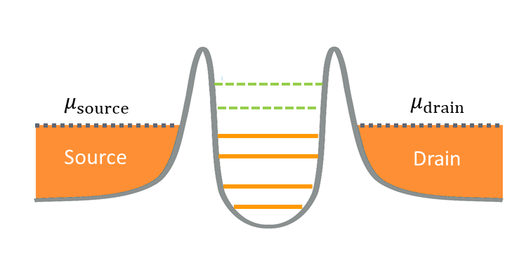
Fig. 8.1 A single quantum dot structure displaying Coulomb blockade.
The Coulomb blockade phenomenon is illustrated in Fig. 8.1. The horizontal lines within the potential well illustrate the chemical potentials of the quantum dot, i.e. the energy required to add an electron to this system. The orange regions on the side represent electron reservoirs at a source and a drain, with the highest occupied state of these reservoirs corresponding to the Fermi energy at zero temperature. In the sequential tunneling regime, for current to flow through the quantum dot, an electron from the source must first tunnel into the dot and then tunnel into the drain. At sufficiently low temperature, this can only be achieved if a chemical potential of the dot lies within the energy bias window between the source and drain chemical potentials. In all other cases, current will be blocked because there is no available quantum-dot state that allows tunneling to happen while conserving energy.
The energy-level structure of a quantum dot can often be shifted by applying
a potential on some gate. In Lever arm theory, we have seen that in the
linear regime, the gate potential and quantum-dot energy levels are related by
the lever arm \(\alpha\). Such a lever arm may be entered into the
many-body Solver
through the optional argument alpha of the class constructor. A gate bias
\(\varphi_\mathrm{bias}\) with respect to a reference configuration in
which the many-body solver is run (and initial chemical potentials calculated)
then shifts the chemical potentials by
\(-e\alpha \varphi_\mathrm{bias}\), as seen in
Eq. (6.1). Compared with the reference configuration (in which
\(\varphi_\mathrm{bias}\equiv 0\)), current is expected to flow through
the device at weak source–drain bias when
We thus expect to see a peak in current associated with every distinct
electron number \(N\) as \(\varphi_\mathrm{bias}\) is swept.
These peaks are called Coulomb peaks; their positions are stored in the
coulomb_peak_pos
attribute of the device object after running the
solve method of the many-body
Solver class.
Particle density
The particle density associated with each many-body eigenstate may be obtained
using the
get_many_body_density
method of the
Device class
(see API Reference).
The electron density in a many-body eigenstate \(|\psi\rangle\) is given by
where \(j\) runs over all single-particle basis states (including the degeneracy index) and \(\langle \hat O\rangle_\psi\equiv \langle\psi|\hat O|\psi\rangle\) is the expectation value of operator \(\hat O\) in state \(|\psi\rangle\).
A simplified many-body Hamiltonian: The Fermi–Hubbard model
For weakly overlapping basis states, Eq. (8.5) reduces to
where we have introduced the particle number operators
In addition, in Eq. (8.15), we have introduced the Coulomb interaction energies \(U_i\) and \(V_{ij}\), which are related to the Coulomb integrals defined in Eq. (8.6) by
The main advantage of using Eq. (8.15) instead of Eq. (8.5) to model Coulomb interactions is that for a basis set containing \(n_\mathrm{states}\) single-particle orbitals, the number of Coulomb integrals to evaluate scales like \(\mathcal O(n_\mathrm{states}^2)\) instead of the more expensive \(\mathcal O (n_\mathrm{states}^4)\) scaling achieved when including overlap terms.
Relevant device attributes
Parameter |
Symbol |
QTCAD name |
Unit |
Default |
Setter |
Confinement potential |
\(V\) |
|
J |
0 |
|
External confinement potential |
\(V_\mathrm{ext}\) |
|
J |
0 |
|
Inverse effective mass tensor |
\(\mathbf M^{-1}_e\) |
|
1/kg |
See note |
Through |