11. The nonequilibrium Green’s function (NEGF) formalism

In the previous section, we saw how the QTCAD junction module can be used to model transport through quantum dots (or other systems with strong confinement) in the sequential tunneling and Coulomb blockade regimes. Importantly, the junction module can thus be used to compute charge-stability diagrams. A drawback of the junction module is that it cannot model other regimes of charge transport, such as thermionic emission or direct source-to-drain tunneling. Furthermore, within the featureless approximation or using the particle addition spectrum, predictions that can be made for the current and conductivity are limited to the position and shape of peaks and plateaus associated with charge transitions; the absolute magnitude of the current or conductivity cannot be predicted from first principles within these approximations. The WKB approximation can be used to make more complete quantitative predictions of the current and conductivity in the sequential tunneling regime, but this approximation relies on potential separability and on the choice of a linecut through which most of the current is expected to flow. These two assumptions are fairly restrictive.

In this section, we will introduce the theoretical formalism underlying QTCAD’s nonequilibrium Green's function (NEGF) module. This formalism can capture nonequilibrium quantum statistics phenomena and model both classical transport (such as thermionic emission above a potential barrier [PHZ+22]) and quantum transport (such as tunneling under a potential barrier [PHZ+22] and conductance quantization [PFP+23]) in devices with arbitrary geometry, material composition, and subject to an arbitrary temperature and external biases. Compared to the junction module, the main shortcoming of the QTCAD NEGF module is that it ignores electron–electron (or hole–hole) interactions, and thus cannot capture Coulomb blockade phenomena. This section will start out with a presentation of the basic theoretical underpinnings and assumptions made in the NEGF formalism. We will then show how charge density and electric potential may be modeled in a quantum device under nonequilibrium conditions through NEGF–Poisson simulations. Finally, we will present how to compute the electric current, density of states, and other relevant physical quantities from Green’s functions.

Basic physical picture of nonequilibrium quantum statistics and transport in the NEGF formalism

Note

The QTCAD NEGF module can only model one type of carrier at a time: electrons or holes. For simplicity, the discussions throughout this section will assume that electrons are being modeled. It should be understood that the discussion applies for holes as well after minor adjustments. Also note that the modeling of holes follows the conventions laid out in QTCAD convention for holes.

By assumption, the systems modeled by the QTCAD NEGF module include:

• a central region, represented by a QTCAD Device object;

• connected to the central region, a source and a drain, namely two semi-infinite thermal reservoirs that maintain thermal equilibrium and may supply and absorb limitless charge and/or energy to and from the central region; note that the QTCAD NEGF module internally handles the source and drain; users need not construct them separately from their Device object.

Such a system is illustrated below.

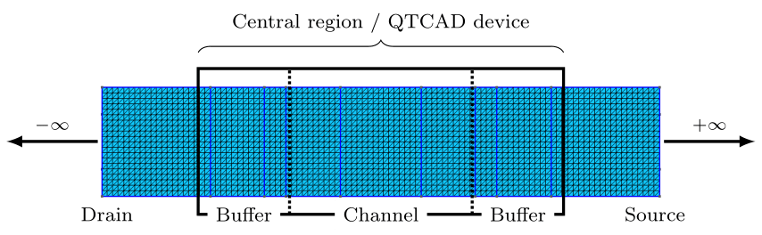
Fig. 11.1 Diagram of a two-probe system within the NEGF formalism.

Importantly, a drain–source bias \(V_{DS}\) may be applied, in which case the drain Fermi level is shifted relative to the source Fermi level (assuming a grounded source). In response to this bias, an electric current flows between the source and drain. Supriyo Datta paints a particularly intuitive picture explaining how this current arises: “Each contact [i.e., the source and drain] seeks to bring the [central region] into equilibrium with itself. The source keeps pumping electrons into it, hoping to establish equilibrium. But equilibrium is never achieved as the drain keeps pulling electrons out in its bid to establish equilibrium with itself. The channel is thus forced in a balancing act between two reservoirs with different agendas and this sends it into a nonequilibrium state intermediate between what the source would like to see and what the drain would like to see.” [Dat05]

Furthermore, while the NEGF formalism explicitly considers the influence of the source and drain on the central region (e.g. through injection of charge from the source/drain into the central region), it cannot model the influence of the central region on the source and drain. For example, the NEGF formalism cannot capture the Coulomb repulsion/attraction induced by a large charge in the central region in the regions of the source/drain neighboring the central region. This is because an assumption underlying the NEGF formalism is that the source and drain are thermal baths with uniform physical properties (such as constant electric potential). For this assumption to be true, buffer regions need to be included in the central region near boundaries with the source/drain (Fig. 11.1). The buffer regions must have the same geometry, material composition, and doping as the source/drain. They need to be sufficiently long to ensure that they are not electrostatically affected by the central region. In other words, the buffer regions serve as transition regions between the central region and the source/drain; in particular, the electric potential in the buffer regions should gradually plateau to a constant value near interfaces with the source/drain.

The retarded Green’s function and other fundamental quantities

The central mathematical object in the NEGF formalism is the retarded Green’s function, which is defined as [Dat97]

(11.1)\[\begin{split}\mathcal{G}^r (E) = \lim\limits_{\substack{\eta\to 0 \\ \eta>0}} \left[(E+i\eta)I - H -\Sigma^r_S (E) - \Sigma^r_D (E)\right]^{-1}\,,\end{split}\]

where \(E\) is the electronic energy, \(I\) is the identity operator, \(H\) is the central region Hamiltonian, and \(\Sigma^r_{S,D}\) are the source and drain retarded self energies. The central region Hamiltonian is computed using the same models as in Schrödinger solvers (namely effective-mass models for electrons and \(\mathbf{k}\cdot\mathbf{p}\) models models for holes). The self energies describe the coupling of the source and drain with the central region. In general, the retarded self energies are complex-valued. Loosely speaking, their imaginary parts impart on the eigenstates of \(H\) a finite lifetime, while their real parts impart shifts to the eigenenergies of \(H\). In QTCAD, the retarded self energies are computed using the elements of \(H\) corresponding to nodes in proximity with the interfaces with the source and drain. It is also worth noting that the limit appearing in Eq. (11.1) is not explicitly evaluated in QTCAD. Rather, the parameter \(\eta\) is fixed to a small value above zero.

Several important quantities may be constructed from the retarded Green’s function and retarded self energies, including the advanced Green’s function,

(11.2)\[\mathcal{G}^a = \left[\mathcal{G}^r\right]^{\dagger}\,,\]

the advanced source and drain self energies,

\[\Sigma^a_{S,D} = \left[\Sigma^r_{S,D}\right]^{\dagger}\,,\]

the source and drain broadening functions,

\[\Gamma_{S,D} = i\left(\Sigma^r_{S,D}-\Sigma^a_{S,D}\right)\,,\]

and the lesser self energy,

\[\Sigma^{<} = i\Gamma_S f_S + i\Gamma_D f_D\,,\]

where \(f_{S,D}\) are the source and drain Fermi–Dirac distribution,

(11.3)\[f_{S,D} = \frac{1}{1+\exp\left(\frac{E-E_{F_{S,D}}}{k_B T}\right)}\,,\]

\[\]

with Fermi levels given by \(E_{F_S}\) and \(E_{F_D}\), respectively. Note that the Fermi levels are related to the drain–source voltage, \(V_{DS}=V_D-V_S\), through

\[E_{F_D} = E_{F_S} - e V_{DS}\,,\]

where \(V_{S,D}\) are the biases applied on the source and drain and \(e>0\) is the elementary charge. Also note that in Eqs. (11.2) to (11.3), the dependence on \(E\) has not been written out explicitly to lighten the notation.

NEGF–Poisson simulations

Calculation of charge density

Having established some of the most fundamental mathematical objects of the NEGF formalism, we may now define the lesser Green’s function through the Keldysh equation [Dat97]

\[\mathcal{G}^{<} = \mathcal{G}^r \Sigma^{<} \mathcal{G}^a\,.\]

Thanks to the Hamiltonian, self energies, and Fermi–Dirac distribution functions that (implicitly) enter its definition, the lesser Green’s function contains information about the energy eigenstates of the central region, their coupling to the leads, as well as their occupation. Provided that the Hamiltonian and self energies are expressed in the real-space basis (with positions labeled by \(\mathbf{r}\)), the elements of the lesser Green’s function may be expressed as \(\mathcal{G}^{<}(\mathbf{r},\mathbf{r}^{\prime}, E)\). The electron density per unit volume is then computed by integrating the diagonal elements of the lesser Green’s function:

(11.4)\[n(\mathbf{r})=\Re\left[\frac{i}{2\pi} \int\limits_{-\infty}^{\infty} \mathcal{G}^{<}(\mathbf{r},\mathbf{r}^{\prime}=\mathbf{r}, E) dE \right]\,.\]

Note that, in general, \(\mathcal{G}^{<}(\mathbf{r},\mathbf{r}^{\prime},E)\) exhibits singularities and discontinuities for \(E\in\mathbb{R}\) which make it numerically challenging to integrate over \(\mathbb{R}\). Instead, the residue theorem is harnessed to re-write Eq. (11.4) as an integral over a complex contour on which \(\mathcal{G}^{<}(\mathbf{r},\mathbf{r}^{\prime},E)\) exhibits fewer singularities and discontinuities; specifically, the QTCAD NEGF module uses the complex contour defined in Ref. [BMOrdejon+02]. Furthermore, QTCAD uses an adaptive integration algorithm to perform this contour integral, thereby leading to accurate evaluations of the charge density.

Self-consistent, iterative solver

We are now ready to describe the Poisson equation that is solved by the QTCAD NEGF–Poisson Solver:

(11.5)\[ \begin{align}\begin{aligned}&-\nabla\cdot\left(\varepsilon\nabla\varphi\right) = \rho\,,\\&\rho = e(-n+N_{+}-N_{-})+\rho_0\,,\end{aligned}\end{align} \]

where, as in Poisson solvers, \(\varepsilon\) is the dielectric permittivity, \(\varphi\) is the electric potential, \(\rho\) is the charge density, \(N_{+,-}\) are the densities of ionized donors and acceptors, and \(\rho_0\) is the fixed background volume charge density. The electron density, \(n\), is defined in Eq. (11.4).

Note

When the considered carriers are holes, the charge density term in Eq. (11.5) is instead given by \(\rho = e(p+N_{+}-N_{-})+\rho_0\), where \(p\) is the hole density computed through the right-hand side of Eq. (11.4).

Note that the central region Hamiltonian \(H\) depends on the electric potential \(\varphi\); see, e.g., Eqs. (3.1), (2.1), and (2.2). Therefore, Eq. (11.5) is a nonlinear equation. In QTCAD, this equation is solved via a self-consistent, iterative procedure whereby:

• An initial guess for the electric potential \(\varphi\) is produced; by default, the solution to the linear Poisson equation is used (i.e. the solution to Eq. (11.5) with \(\rho=0\)).

• The electron density is then computed through Eq. (11.4).

• The electric potential is updated by solving Eq. (11.5).

• The last two steps are iterated until variations in the electric potential between the current iteration and the last iteration fall below a predefined tolerance, at which point the NEGF–Poisson algorithm is deemed to have converged.

Specifically, the convergence criterion for NEGF–Poisson simulations is:

(11.6)\[\left\Vert\ \varphi_{\textrm{current}} - \varphi_{\textrm{previous}} \right\Vert_{\infty} \leq \varphi_{\epsilon}\,,\]

where \(\varphi_{\textrm{current}}\) (\(\varphi_{\textrm{previous}}\)) is the electric potential for the current (previous) iteration and \(\varphi_{\epsilon}\) is the convergence criterion (by default set to \(10^{-5}~\textrm{V}\)).

Boundary conditions

The possible boundary conditions for the Poisson equation (Eq. (11.5)) include all of those described in Boundary conditions. In addition, for a QTCAD NEGF–Poisson simulation, exactly two surfaces (the source and drain boundaries) need to be assigned a so-called quantum lead boundary condition using the new_quantum_lead_bnd method. This method takes as its second argument a boolean, essential. If essential=False, the boundary is treated as a natural boundary condition. If essential=True, not unlike an Ohmic boundary condition, the potential is determined by imposing charge neutrality,

(11.7)\[- n + N_+ - N_- = 0\,,\]

with the caveat that \(n\) is computed in terms of the 1D bandstructure of the semi-infinite source/drain and the source/drain Fermi level \(E_{F_{S,D}}\). It is recommended to use essential=False whenever possible, namely whenever the device has at least one essential boundary.

In addition, at boundaries or regions with perfect insulators or ideal oxides, the electron density \(n\) (Eq. (11.4)) is set to zero.

Note

When the considered carriers are holes, Eq. (11.7) is replaced by \(p + N_+ - N_- = 0\), where \(p\) is the hole density computed through the right-hand side of Eq. (11.4). In addition, it is the hole density \(p\) that is set to zero at boundaries or regions with perfect insulators.

Calculation of drain–source current, density of states, and other relevant quantities

Transmission function and drain–source current

Having obtained the electric potential throughout the device using NEGF–Poisson simulations, the central region’s Hamiltonian \(H\) and thus the retarded Green’s function \(\mathcal{G}^r\) are now known without ambiguity. We are thus in a position to compute the drain–source current. To do so, we first define the transmission function [Dat97],

(11.8)\[\overline{T}(E) = \mathrm{Tr} \left[ \Gamma_D \mathcal{G}^r \Gamma_S \mathcal{G}^a\right]\,.\]

The drain–source current may then be computed through the Landauer–Büttiker formula:

(11.9)\[I_{DS} = \frac{e}{h} \int\limits_{-\infty}^{\infty} \overline{T}(E) \left[ f_S(E) - f_D(E)\right]dE\,.\]

This assumes that transport is coherent, namely that electrons flow between the source and drain in independent energy modes. In particular, this excludes transport with inelastic scattering (e.g. electron–phonon scattering). Under this assumption, loosely speaking, the transmission function at energy \(E\) can be thought of as the product of (A) the number of conduction modes between the source and drain at energy \(E\) and (B) the transmission probability between the source and drain at energy \(E\) [Dat05].

It may be observed that \(I_{DS}\geq 0\) when \(V_{DS}>0\), since \(\overline{T}(E)\geq 0\) for all \(E\). In addition, note that the transmission function \(\overline{T}(E)\) may be computed and plotted using the plot_transmission method, while the drain–source current \(I_{DS}\) may be computed and plotted using the get_current and get_current_adaptive methods. In addition, the plot_spectral_current method can be used to compute and plot the spectral current, namely the integrand appearing in Eq. (11.9):

(11.10)\[i_{DS}(E) = \frac{e}{h} \overline{T}(E) \left[ f_S(E) - f_D(E)\right]\,.\]

Density of states and local density of states

The spectral function is an important quantity within the NEGF formalism, as it carries information about the available states of the central region and their lifetimes. It is simply defined as

\[A = i (\mathcal{G}^r - \mathcal{G}^a)\,.\]

By taking the trace of the spectral function, we may compute the density of states (DOS) of the central region [Dat97]:

(11.11)\[\mathrm{DOS}(E) = \frac{1}{2\pi} \mathrm{Tr}\left[A(E)\right]\,.\]

The DOS may be computed and/or plotted using the plot_dos method.

Furthermore, the diagonal elements of the spectral function (in its real-space representation) are proportional to the local density of states (LDOS) [Dat97]:

(11.12)\[\mathrm{LDOS}(\mathbf{r},E) = \frac{1}{2\pi} A(\mathbf{r}, \mathbf{r}^{\prime}=\mathbf{r}, E)\,.\]

The LDOS may be computed and/or plotted using the plot_ldos method.

In a similar vein, the spectral density, namely the energy-resolved and spatially-resolved carrier density, may be computed from the lesser Green’s function [Dat97]:

(11.13)\[n(\mathbf{r}, E) = - i \mathcal{G}^{<}(\mathbf{r}, \mathbf{r}^{\prime}=\mathbf{r}, E)\,.\]

This quantity may be computed and/or plotted using the plot_spectral_density method.