1. Quantum transport—Master equation
1.1. Requirements
1.1.1. Software components
QTCAD
1.1.2. Python script
qtcad/examples/tutorials/gaafet_diamond.py
1.1.3. References
1.2. Briefing
In this tutorial, we demonstrate how to perform a quantum transport calculation. In this calculation, we solve the master equation that describes transport from a source to a drain due to sequential tunneling through a confined (quantum dot) region. The eigenstates of the quantum dot region that appear in the master equation are obtained by exact diagonalization of the many-body Hamiltonian of conduction electrons in the truncated basis formed by a few single-particle eigenstates. These single-particle eigenstates are found by solving the Schrödinger equation in the dot region. This method yields the current flowing through the device as a function of applied source–drain and gate potentials, and thus gives us access to the position of Coulomb peaks, allowing us to draw charge-stability diagrams.
1.3. Setting up the device
1.3.1. Header
In addition to what has already been invoked in
Poisson and Schrödinger simulation of a GAAFET, here we also need to import relevant classes and
functions from the
mastereq
and junction modules.
import numpy as np
from matplotlib import pyplot as plt
import pathlib
from progress.bar import ChargingBar as Bar

from qtcad.device import constants as ct
from qtcad.device import materials as mt
from qtcad.device.mesh3d import Mesh
from qtcad.device import io
from qtcad.device import Device
from qtcad.device.schrodinger import Solver
from qtcad.device.many_body import SolverParams

from qtcad.transport.mastereq import seq_tunnel_curr
from qtcad.transport.junction import Junction
Junction: Class that contains all information about the transport system, i.e. the two leads (source and drain), and the quantum-dot system.seq_tunnel_curr: Function to compute transport properties
1.3.2. Load data
Here we assume that a device structure has already been treated, and
that a single-particle confinement potential was found and saved on our
disc. For conduction electrons, this corresponds to the conduction band
edge. In this tutorial, we reuse the result from Poisson and Schrödinger simulation of a GAAFET. Indeed, the conduction band edge
(along with several other variables) was saved in .hdf5 format.
We will thus load the mesh, create an empty device, and load the only quantity that we need (the conduction band edge) for the quantum transport calculation.
# Load the mesh
script_dir = pathlib.Path(__file__).parent.resolve()
path_mesh = script_dir / "meshes/" / "gaafet.msh"
path_in = script_dir / "output/" / "gaafet.hdf5"

mesh = Mesh(1e-9, str(path_mesh))
d = Device(mesh=mesh, conf_carriers="e")
d.new_region('channel_ox',mt.SiO2)
d.new_region('source_ox',mt.SiO2)
d.new_region('drain_ox',mt.SiO2)
d.new_region('channel', mt.Si)
d.new_region('source', mt.Si, pdoping=5e20*1e6, ndoping=0)
d.new_region('drain', mt.Si, pdoping=5e20*1e6, ndoping=0)
d.V = io.load(str(path_in), var_name="EC") * ct.e
The last line sets the electron potential energy to be the conduction band edge calculated in the previous tutorial. Note that we multiply by the fundamental electric charge to obtain SI units, since energies obtained in the previous tutorial were saved using \(\textrm{eV}\) units.
1.3.3. Solving Schrödinger’s equation for single electrons
The first step is to solve the single-body Schrödinger’s equation for
the loaded potential energy, stored in the device attribute d.V. The
resulting envelope functions will then be used as a basis set to solve
the many-body problem, including Coulomb interaction between electrons.
# Solve Schrodinger's equation for single electrons
s = Solver(d)
s.solve()
1.3.4. Initializing a Junction object
A Junction
object is initialized through the following interface
# Many-body solver parameters
solver_params = SolverParams()
solver_params.num_states=2          # Number of basis states to keep
solver_params.n_degen=2             # spin degenerate system

# Initialize junction
jc = Junction(d, many_body_solver_params=solver_params)
It is recommended to set the parameters of the many-body solver that lives
inside the Junction object
using a many-body SolverParams
object that is passed as an optional argument to the
Junction
constructor. For example, parameters that are often tuned this way are:
num_states: Number of one-particle eigenstates to be included in the many-body basis set. The Fock-space dimension in the following many-body simulation is thus 2^(num_states*spin)
n_degen: The degeneracy of each level. In this case we set
n_degen = 2to account for the spin degeneracy.
The initialization procedure may take a while since the program will set up the many-body Hamiltonian and diagonalize it. The many-body eigenenergies can be extracted via
jc.get_all_eig_energies()
After initialization one may still be able to set certain parameters through Junction-class methods, such as
jc.set_temperature(0.1)   # set temperature in unit of K
jc.setVg(0.1)  # set gate voltage in volts
jc.setVs(0.1)  # set source voltage in volts
jc.setVd(0.1)  # set drain voltage in volts
The source–drain voltages are assumed to rigidly shift the chemical potentials of corresponding reservoirs, and applying a gate voltage effectively shifts the entire energy spectrum of the device by \(-e V_g\), corresponding to an ideal lever arm \(\alpha = 1\).
Note that the electrostatics is not recalculated when we manually set
these potential parameters. However, the actual lever arm for a given
device geometry may be accounted for by setting the keyword argument
alpha of the Junction
constructor to the chosen value (different
from the default value of 1). The single-particle eigenenergies are then
shifted by \(-e \alpha V_g\) when applying a gate potential \(V_g\).
The lever arm \(\alpha\) may easily be found by finding the single-particle
eigenenergies as a function of \(e V_g\), and fitting the result to a
straight line, as see in Calculating the lever arm of a quantum dot.
The slope of this line then gives \(-\alpha\).
Note
As explained in Many-body analysis of a GAAFET, the gate bias is expressed
with respect to the reference gate potential, i.e., the potential applied
on the gate boundary condition when solving Poisson’s equation which lead
to the confinement potential used here. For example, if the reference gate
potential was \(V_\mathrm{GS}=0.5\;\mathrm V\), the bias of
\(0.1\;\mathrm V\) applied here through the
setVg method corresponds to
a physical gate potential of
\(0.5\;\mathrm V+0.1\;\mathrm V=0.6\;\mathrm V\).
This approach enables to produce charge stability diagrams even for
confinement potentials that were loaded from previous simulations, or
from analytic confinement potentials that are not the numerical solution
of the electrostatics of a realistic device.
1.4. Transport calculation
To calculate transport currents and statistical distribution we invoke
the seq_tunnel_curr
function
Il,Ir,prob = seq_tunnel_curr(jc)
Il: charge current from source
Ir: charge current from drain. The relationship
Il+Ir=0 should be respected.prob: occupation probability for each many-body state in the stationary (steady-state) regime.
We note that the currents Il and Ir are evaluated assuming that the
single-particle broadening functions appearing in the master equation rates
are constant over all possible pairs of single-particle eigenstates (see
The sequential tunneling master equation and Broadening function: featureless approximation sections of our
theory documentation). This has the benefit of speeding up calculations
which involve solving master equations, while giving a qualitative
understanding of different transport phenomena, e.g. Coulomb Blockade.
However, the currents themselves are not meant to be quantitatively
accurate. In this tutorial we wish to produce Coulomb diamonds.
To do this we sweep the source/drain and gate voltages over a range.
jc.set_temperature(1)   # set temperature in unit of K

# Get Coulomb diamonds
v_gate_rng = np.linspace(0.45, 0.85, num=100)
v_source_rng = np.linspace(-0.08, 0.08, num=100)
diam = np.zeros((v_gate_rng.size, v_source_rng.size), dtype=float)

number_grid_points = v_gate_rng.size * v_source_rng.size # number of sampled grid points
progress_bar = Bar("Computing charge stability diagram", max = number_grid_points) # initialize progress bar

# loop over gate voltage
for i, v_gate in enumerate(v_gate_rng):
    # Set gate voltage
    jc.setVg(v_gate)
    # loop over source/drain voltage
    for j, v_source in enumerate(v_source_rng):
        # Set source and drain voltages
        jc.setVs(v_source)
        jc.setVd(-v_source) # Drain voltage opposite in sign to source

        # Compute currents
        Il,Ir,prob = seq_tunnel_curr(jc)    # transport calculation
        diam[i,j] = Il

        progress_bar.next()

progress_bar.finish()
This procedure yields a 2d array diam which stores the current
obtained under every sampled voltage configuration. While the first
index of the array corresponds to gate potentials, the second index
corresponds to source–drain biases. Note that, to keep track of the progress
of the calculation of this charge-stability diagram, we have instantiated a
progress bar progress_bar as implemented in the progress.bar Python
library.
We get a quantity proportional to the differential conductance (derivative of the current with respect to source–drain bias) by taking differences of the current
# differential conductance
diam_diff_cond = np.abs(diam[:,1:] - diam[:,:-1])
Note
The convention for the sign of the currents is the following: a positive current means conventional (positive) charge tunneling from a lead to the dot. Such a current is expressed in Ampere units. Note that within this convention, when a net current is flowing through the device, individual currents associated with each lead will have opposite signs.
1.4.1. Plotting results
Finally, we plot diam_diff_cond to visualize the Coulomb diamonds.
# plot results
fig, axs = plt.subplots()
axs.set_ylabel('$V_s(V)$',fontsize=16)
axs.set_xlabel('$V_g(V)$',fontsize=16)
diff_cond_map = axs.imshow(np.transpose(diam_diff_cond), interpolation='bilinear',
         extent=[v_gate_rng[0], v_gate_rng[-1],
                  v_source_rng[-2], v_source_rng[0]], aspect="auto")
fig.colorbar(diff_cond_map, ax=axs, label="Differential conductance (arb. units)")
fig.tight_layout()
plt.show()
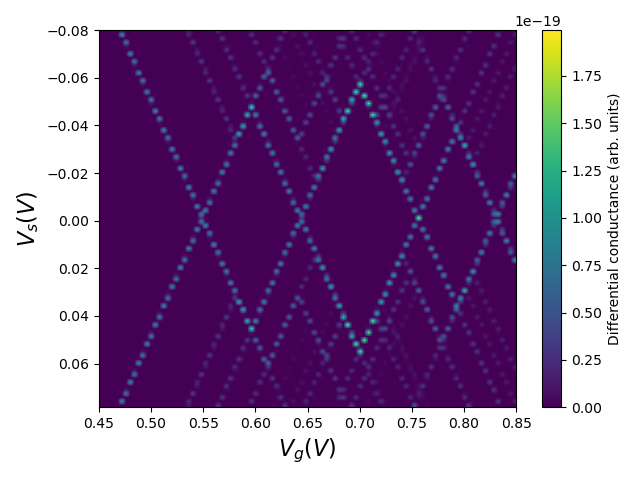
Fig. 1.4.2 Coulomb diamonds
The diamonds in the above diagram manifest the Coulomb blockade regions in which the source–drain and gate voltage configuration determines a quantized electron occupation number due to Coulomb repulsion. Recall that the gate bias expressed on the \(x\) axis of this plot should be understood as given with respect to the reference gate potential applied at the boundary when solving Poisson’s equation. Therefore, for the confinement potential used here, which was loaded from the Poisson and Schrödinger simulation of a GAAFET tutorial, an offset of \(V_\mathrm{GS}=0.5\;\mathrm V\) should be added to the \(x\) axis to plot the charge stability diagram as a function of the true applied potential at the gate.
In the next tutorial (Quantum transport—WKB approximation), we will perform a more involved transport calculation using the WKB approximation. We expect this more involved calculation to be more quantitatively accurate than the procedure presented here.
1.5. Full code
__copyright__ = "Copyright 2024, Nanoacademic Technologies Inc."

import numpy as np
from matplotlib import pyplot as plt
import pathlib
from progress.bar import ChargingBar as Bar
from qtcad.device import constants as ct
from qtcad.device import materials as mt
from qtcad.device.mesh3d import Mesh
from qtcad.device import io
from qtcad.device import Device
from qtcad.device.schrodinger import Solver
from qtcad.device.many_body import SolverParams
from qtcad.transport.mastereq import seq_tunnel_curr
from qtcad.transport.junction import Junction

# Load the mesh
script_dir = pathlib.Path(__file__).parent.resolve()
path_mesh = script_dir / "meshes/" / "gaafet.msh"
path_in = script_dir / "output/" / "gaafet.hdf5"

mesh = Mesh(1e-9, str(path_mesh))
d = Device(mesh=mesh, conf_carriers="e")
d.new_region('channel_ox',mt.SiO2)
d.new_region('source_ox',mt.SiO2)
d.new_region('drain_ox',mt.SiO2)
d.new_region('channel', mt.Si)
d.new_region('source', mt.Si, pdoping=5e20*1e6, ndoping=0)
d.new_region('drain', mt.Si, pdoping=5e20*1e6, ndoping=0)
d.V = io.load(str(path_in), var_name="EC") * ct.e

# Solve Schrodinger's equation for single electrons
s = Solver(d)
s.solve()

# Many-body solver parameters
solver_params = SolverParams()
solver_params.num_states=2          # Number of basis states to keep
solver_params.n_degen=2             # spin degenerate system

# Initialize junction
jc = Junction(d, many_body_solver_params=solver_params)

jc.set_temperature(1)   # set temperature in unit of K

# Get Coulomb diamonds
v_gate_rng = np.linspace(0.45, 0.85, num=100)
v_source_rng = np.linspace(-0.08, 0.08, num=100)
diam = np.zeros((v_gate_rng.size, v_source_rng.size), dtype=float)

number_grid_points = v_gate_rng.size * v_source_rng.size # number of sampled grid points
progress_bar = Bar("Computing charge stability diagram", max = number_grid_points) # initialize progress bar

# loop over gate voltage
for i, v_gate in enumerate(v_gate_rng):
    # Set gate voltage
    jc.setVg(v_gate)
    # loop over source/drain voltage
    for j, v_source in enumerate(v_source_rng):
        # Set source and drain voltages
        jc.setVs(v_source)
        jc.setVd(-v_source) # Drain voltage opposite in sign to source

        # Compute currents
        Il,Ir,prob = seq_tunnel_curr(jc)    # transport calculation
        diam[i,j] = Il

        progress_bar.next()

progress_bar.finish()

# differential conductance
diam_diff_cond = np.abs(diam[:,1:] - diam[:,:-1])

# plot results
fig, axs = plt.subplots()
axs.set_ylabel('$V_s(V)$',fontsize=16)
axs.set_xlabel('$V_g(V)$',fontsize=16)
diff_cond_map = axs.imshow(np.transpose(diam_diff_cond), interpolation='bilinear',
         extent=[v_gate_rng[0], v_gate_rng[-1],
                  v_source_rng[-2], v_source_rng[0]], aspect="auto")
fig.colorbar(diff_cond_map, ax=axs, label="Differential conductance (arb. units)")
fig.tight_layout()
plt.show()