1.5. Band structure calculation
In this section, I show how to perform a band-structure calculation.
Copy the following input file and save it to a text file named
si_bs.txt.
info.calculationType = 'band-structure'
info.savepath = 'results/si_bs'
atom.element = [1 1]
atom.xyz = 10.25*[0 0 0;0.25 0.25 0.25]
domain.latvec = 10.25*[0.0 0.5 0.5;0.5 0.0 0.5;0.5 0.5 0.0]
domain.lowres = 0.5
element.species = 'si'
element.path = './Si_TM_LDA.mat'
rho.in = 'results/si_scf'
Then pass it to RESCU and execute the program as follows
rescu -i si_bs.txt;
The band-structure calculation input file is similar to the
self-consistent calculation input except for the keywords
info.calculationType which value changed to band-structure and
rho.in which points to the results of the self-consistent
calculation. In this example, RESCU recognizes the face-centered cubic
lattice, defines a line sampling the irreducible Brillouin zone edges
and determines the number of k-points required to achieve the default
k-point resolution. Arbitrary k-points lines are defined via the
kpoint.sympoints keyword. It must be a cell array containing k-point
labels or direct coordinates, and the number of k-points can be adjusted
using kpoint.gridn. For example,
kpoint.sympoints = {’G’,[0,0,0.5],’L’,[0.625,0.25,0.625]}. The band
structure for the auto-generated line is found in
Fig. 1.5.1. The FCC irreducible Brillouin zone
edges cannot be visited in a single continuous line, and hence the
segment U-X is thus appended to the first k-point line.
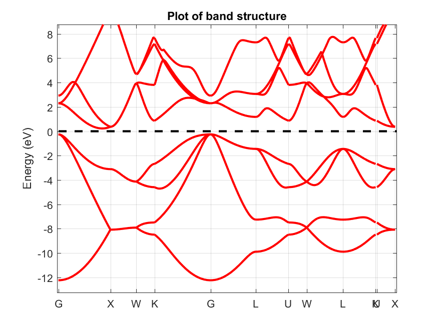
Fig. 1.5.1 Band structure of bulk silicon.