5. Maxwell eigenmode extraction for an Xmon qubit: inductor ports and EPR analysis

5.1. Requirements

5.1.1. Software components

• QTCAD

• Gmsh

5.1.2. Geometry file

• qtcad/examples/tutorials/meshes/xmon.py

5.1.3. Python script

• qtcad/examples/tutorials/maxwell_xmon.py

5.1.4. References

• Maxwell eigenmode extraction of a coplanar waveguide resonator with adaptive meshing

• Capacitance matrix extraction for an Xmon qubit

• Inductor boundaries (API reference)

• Energy-participation-ratio method

5.2. Briefing

In this tutorial, we explain how to use inductor boundaries in the Maxwell eigenmode Solver. The device considered is the Xmon [BKM+13] from the tutorial Capacitance matrix extraction for an Xmon qubit. Here, an inductor boundary, described in Inductor boundaries (API reference), is associated to the surface representing the Josephson junction; that is, we approximate it as a linear inductor. In general, such an analysis is relevant because the eigenmode extraction involving linearized Josephson circuits is an important step in the energy-participation quantization method [MLM+21]. The last section of this tutorial shows how to post-process the resulting Maxwell eigenmode with the energy-participation-ratio (EPR) module.

5.3. Xmon qubit under consideration

The operation of an Xmon qubit [BKM+13] is based on that of a transmon qubit [KYG+07]. This type of qubit is formed by a capacitor and a Josephson junction in parallel, as illustrated on the left of Fig. 5.3.4.

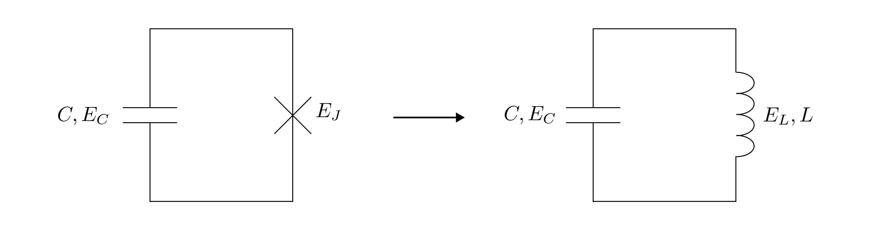
Fig. 5.3.4 Transmon qubit and the linearized LC oscillator approximation.

The Josephson junction is governed by the following equations [BGGW21]:

(5.3.1)\[i_{\text{JJ}}(t) = I_c \sin\left(\dfrac{2 \pi \Phi(t)}{\Phi_0}\right)\]

and

(5.3.2)\[\dfrac{d\Phi}{dt} = v_{\text{JJ}}(t),\]

where \(i_{\text{JJ}}\) and \(v_{\text{JJ}}\) are the current and voltage of the junction respectively and \(I_c\) is the critical current. Also, \(\Phi_0=h/(2e)\) is the superconducting flux quantum and \(\Phi(t)\) is the so-called flux variable, analogous to the magnetic flux in an inductor.

The capacitor and the Josephson junction form a weakly anharmonic oscillator, where, in the classical description, the capacitor charge and the flux variable oscillate around zero. The anharmonicity of the oscillator comes from the nonlinear nature of the Josephson junction, namely the non-linear relation Eq. (5.3.1) between the current and the flux variable.

The transmon exhibits quantized energy levels, with the separation between the first two levels given by [BGGW21]

(5.3.3)\[E_{01} = \sqrt{8 E_C E_J} - E_C,\]

where \(E_C=e^2/(2C)\) is the charging energy [1] and \(E_J = \Phi_0 I_c/(2\pi)\) is the Josephson energy [2].

The anharmonicity of the oscillator manifests itself in the unequal separation between energy levels, and is quantified as \(E_{12}-E_{01} = -E_C\) [BGGW21, KYG+07]. Here, \(E_{ij} \equiv E_j - E_i\) is the energy separation between the energy levels \(i\) and \(j\). For a transmon, the anharmonicity is much smaller than the energy level separation. Nevertheless, it is essential in ensuring that the quantum oscillator stays within the first two energy levels, allowing it to operate as a qubit.

5.3.1. Modeling Josephson junction as an inductor

The Josephson junction can be thought of as a nonlinear inductor, with the inductance given by [BGGW21]

(5.3.4)\[L = \dfrac{\Phi_0^2}{(2 \pi)^2 E_J} \dfrac{1}{\cos(2 \pi \Phi/\Phi_0)}.\]

For small oscillations of \(\Phi\), the Josephson junction can be linearized by setting \(\Phi\) to zero in Eq. (5.3.4), yielding an inductance that is independent of the flux variable:

(5.3.5)\[L \approx \dfrac{\Phi_0^2}{(2 \pi)^2 E_J}.\]

The energy level separation of an LC harmonic quantum oscillator is given by [BGGW21]

(5.3.6)\[E_{01, LC} = \hbar \omega_{LC},\]

where

(5.3.7)\[\omega_{LC} = \dfrac1{\sqrt {LC}}\]

is the resonant angular frequency of the classical LC harmonic oscillator.

5.4. Geometry of the problem

The geometry of the device is the same as in the tutorial Capacitance matrix extraction for an Xmon qubit. The layout and dimensions were kindly provided by Christopher Xu from Red Blue Quantum.

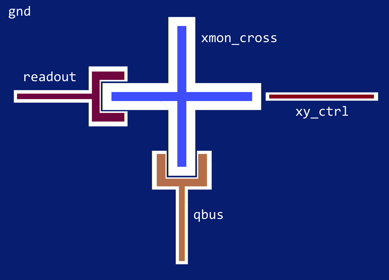
Fig. 5.4.9 Layout of the Xmon.

5.5. Setting up the device and finding the Maxwell eigenmodes

The procedure for finding the Maxwell eigenmodes is similar to that described in the tutorial Maxwell eigenmode extraction of a coplanar waveguide resonator with adaptive meshing, with the additional step of adding the inductor to the device.

5.5.1. Header, input parameters, and file paths

"""
Maxwell eigenmodes for an Xmon with the Josephson junction represented as a linear
inductor.

The layout and dimensions for this example were kindly provided by Christopher Xu from
Red Blue Quantum.

See the following article for more details on the operation of an Xmon qubit coupled to
a readout line, XY control line, and a quantum bus resonator.
    Barends, Rami, et al. "Coherent Josephson qubit suitable for scalable quantum
    integrated circuits." Phys. Rev. Lett., 111.8 (2013): 080502.
"""

from pathlib import Path
import os
from time import time
import numpy as np

# Import relevant modules of QTCAD.
from qtcad.device.maxwell_eigenmode import Solver
from qtcad.device.maxwell_eigenmode import SolverParams
from qtcad.device.device import Device
from qtcad.device.mesh3d import Mesh
from qtcad.device import materials as mt
from qtcad.device import constants as ct

The Solver class contains algorithms needed to find the Maxwell eigenmodes and the SolverParams class can be used to control parameters of the solver.

To proceed, let us define some general variables related to the output directory and files, as well as the mesh:

# Scale in the Gmsh files. That is, Gmsh file coordinates are in μm.
scale = 1e-6

# Directories and file paths.
script_dir = Path(__file__).parent.resolve()
# For mesh and raw geometry files.
input_dir = script_dir / "meshes"
# For results.
result_dir = script_dir / "output" / Path(__file__).stem
# Mesh file.
fpath_mesh = input_dir / "xmon.msh"
# Raw geometry file (needed for adaptive meshing).
fpath_xao = input_dir / "xmon.xao"

# Check if the mesh and raw geometry files exist.
if not os.path.isfile(fpath_mesh) or not os.path.isfile(fpath_xao):
    raise Exception(
        "Please run %s/xmon.py to generate the mesh and raw geometry files."
        % (input_dir)
    )

5.5.2. Loading the initial mesh and defining the device

Next, we parse the mesh file, initialize the device and assign the media to 3D physical groups and boundary conditions to 2D physical groups:

######################################################################################
# Setup the device.
######################################################################################
# Parse the mesh and initialize the device.
mesh = Mesh(scale, fpath_mesh)
dvc = Device(mesh)

material_sub = mt.Si
material_air = mt.vacuum
# Assign media to regions.
dvc.new_region("substrate", material_sub)
dvc.new_region("air", material_air)
# Assign perfect electric conductor boundary condition to all conductors.
dvc.new_pec_bnd("gnd")
dvc.new_pec_bnd("xmon_cross")
dvc.new_pec_bnd("xy_ctrl")
dvc.new_pec_bnd("readout")
dvc.new_pec_bnd("qbus")

Then, we add an inductor to represent the Josephson junction:

# Calculate inductance.
#
# For the expression of the inductance as a function of the flux, see
#   Alexandre Blais, Arne L. Grimsmo, S. M. Girvin, and Andreas Wallraff.
#   Circuit quantum electrodynamics. Rev. Mod. Phys., 93:025005, May 2021.
EJ = 23e9 * ct.h
Phi0 = ct.h / (2 * ct.e)
inductance = Phi0**2 / ((2 * np.pi) ** 2 * EJ)

# Add the inductor.
dvc.new_inductor("jj", inductance, dir="y", length=24e-6, width=24e-6)

Here, when adding the inductor with new_inductor, we specify dir="y" to indicate that the current of the inductor flows between the conductor of the Xmon superconducting island and the ground plane. Currently, we support the orthogonal directions "x", "y" and "z". Also, the dimensions length and width are the dimensions of the boundary of the inductor "jj". They must be passed and, in this example, can be found in the geometry file.

More information on inductor boundaries can be found in Inductor boundaries (API reference).

5.5.3. Creating and running the Maxwell eigenmode solver

######################################################################################
# Setup the solver.
######################################################################################
params = SolverParams()
# Number of modes to find.
params.num_modes = 1
# Adaptive meshing (relative) tolerance on the frequency.
params.tol_rel = 0.03
# Directory where output files will be stored
params.output_dir = result_dir

######################################################################################
# Run the solver (results are stored in the folder specified by params.output_dir).
######################################################################################
slv = Solver(dvc, params, geo_file=fpath_xao)
t0 = time()
slv.solve()
dt = time() - t0
print("Solution completed in %.2f s" % dt)

5.5.4. Extracting further solver results

Next, we can display the computed frequency, along with the analytical frequency of the the LC resonator formed by the Xmon capacitor and the linearized inductor. The latter is computed by dividing Eq. (5.3.7) by \(2 \pi\).

######################################################################################
# Extract additional information from the final results.
######################################################################################

# From the cap_xmon.py tutorial.
capacitance = 1.014e-13

freq_lc = 1 / np.sqrt(inductance * capacitance) / (2 * np.pi)
freq_lc_ghz = freq_lc / 1e9
print(f"Frequency of the LC resonator (analytical): {freq_lc_ghz:.3f} GHz")

freq_ghz = dvc.maxwell_freqs[0] / 1e9
print(f"Frequency of the fundamental mode (computed): {freq_ghz:.3f} GHz")

The resulting frequencies are

Frequency of the LC resonator (analytical): 5.929 GHz
Frequency of the fundamental mode (computed): 5.741 GHz

It should be noted that the LC resonator model is a good reference for comparison, as the size of the device is much smaller than the wavelength of electromagnetic waves at these resonant frequencies [3].

For completeness, we also show the frequency of the original qubit, computed from Eq. (5.3.3):

# Blais et al. (2021).
EC = ct.e**2 / (2 * capacitance)
freq_qbit = (np.sqrt(8 * EC * EJ) - EC) / ct.h
freq_qbit_ghz = freq_qbit / 1e9
print(f"Frequency of the qubit (analytical): {freq_qbit_ghz:.3f} GHz")

Frequency of the qubit (analytical): 5.738 GHz

The resulting fields from the xmon-fields.vtu file are shown in the figures below:

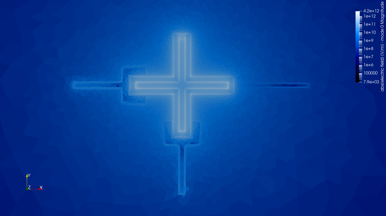
Fig. 5.5.4 Magnitude of the electric field viewed in ParaView. Clip filter at \(z=0\) is used to visualize the field at the level of the the ground plane. The values are displayed in logarithmic scale with the “Black, Blue and White” colour scheme.

Fig. 5.5.5 Magnitude of the magnetic flux density viewed in ParaView. Clip filter at \(z=0\) is used to visualize the field at the level of the the ground plane. The values are displayed in logarithmic scale with the “Black, Blue and White” colour scheme.

5.6. Energy-participation-ratio analysis

The above solution of the linearized-junction problem is a requirement for the use of the EPR method [MLM+21]. As explained in Energy-participation-ratio method, the Josephson potential can be expanded around zero reduced flux. The resulting quadratic term is associated with the linear inductor already used in the Maxwell eigenmode problem, while the leading nonlinear correction comes from the quartic term.

The EPR module uses the solved linear modes to compute the fraction of each mode’s inductive energy stored in each Josephson junction. For mode \(m\) and junction \(j\), this energy participation is

\[p_{mj} = \frac{ U_{Jj,m}^{\mathrm{lin}} }{ U_m^{\mathrm{ind}} },\]

where \(U_{Jj,m}^{\mathrm{lin}}\) is the linear inductive energy stored in the junction and \(U_m^{\mathrm{ind}}\) is the total inductive energy of the mode.

For a mode frequency \(f_m\), this energy participation determines the reduced-flux zero-point fluctuation through

\[\varphi_{mj} = s_{mj} \sqrt{ p_{mj}\frac{h f_m}{2E_{Jj}} },\]

where \(s_{mj}=\pm 1\) is set by the current orientation.

From these quantities, QTCAD^® extracts dressed frequencies, Kerr coefficients and the anharmonicity of the qubit mode via EPRAnalysis, which must be used after the Maxwell eigenmode solver has been run. The usage of EPRAnalysis is demonstrated below.

5.6.1. Importing the EPR classes and identifying junctions

In addition to the modules imported earlier, let us import the relevant classes for EPR analysis: EPRAnalysis and JunctionSpec.

from qtcad.device.epr import EPRAnalysis, JunctionSpec

The JunctionSpec object identifies one Josephson junction boundary. Its boundary name must match the physical group’s name used to set up the inductor port in the eigenmode solver. In this example, we have a single junction whose boundary name is "jj". Let us then create a list with the junctions on which we would like to run the EPR analysis.

epr_junctions = [JunctionSpec("jj")]

5.6.2. Running the EPR analysis

We can now run the EPR analysis:

######################################################################################
# Solve EPR analysis.
######################################################################################
# The EPR analysis reads the solved Maxwell fields and the current through the
# inductor boundary named "jj", then converts the linear EPR data into
# first-order nonlinear quantities such as the dressed frequency, zero-point
# fluctuations and anharmonicity.
epr = EPRAnalysis(dvc, epr_junctions).solve()

Here, the first argument is the solved device dvc. The second argument is the list of Josephson junctions to include in the EPR analysis.

Since we only solved for a single Maxwell eigenmode, the resulting arrays will have one mode row and one junction column. For example, epr.participation[0, 0] is the junction participation of the fundamental mode and epr.phi_zpf[0, 0] is the corresponding reduced-flux zero-point fluctuation.

5.6.3. Comparing EPR and analytical quantities

Let us then print a compact comparison table of some relevant quantities of interest. The EPR-specific rows are obtained from the EPRResult returned by solve.

######################################################################################
# EPR results and comparisons with simple analytical estimates.
######################################################################################
rows = [
    ("Frequency of the LC resonator (analytical)", f"{freq_lc / 1e9:.3f} GHz"),
    ("Bare Maxwell frequency (computed)", f"{epr.bare_frequencies[0] / 1e9:.3f} GHz"),
    ("Dressed qubit frequency (EPR)", f"{epr.dressed_frequencies[0] / 1e9:.3f} GHz"),
    ("Frequency of the qubit (analytical)", f"{freq_qbit / 1e9:.3f} GHz"),
    ("Junction participation", f"{epr.participation[0, 0]:.6f}"),
    ("Reduced flux ZPF", f"{epr.phi_zpf[0, 0]:.6f}"),
    ("Anharmonicity", f"{epr.anharmonicity[0] / 1e6:.3f} MHz"),
]

# Display data as a table.
header = f"{'Quantity':<45} | {'Value':>15}"
print("\n" + header)
print("-" * len(header))
for label, value in rows:
    print(f"{label:<45} | {value:>15}")

We obtain:

Quantity                                      |           Value
---------------------------------------------------------------
Frequency of the LC resonator (analytical)    |       5.929 GHz
Bare Maxwell frequency (computed)             |       5.741 GHz
Dressed qubit frequency (EPR)                 |       5.567 GHz
Frequency of the qubit (analytical)           |       5.738 GHz
Junction participation                        |        0.985469
Reduced flux ZPF                              |        0.350696
Anharmonicity                                 |    -173.948 MHz

Here,

• The bare frequency is the linearized Maxwell eigenfrequency before the quartic Josephson correction.

• The dressed frequency is the first-order EPR frequency after subtracting the Lamb shift associated with the junction nonlinearity.

• The participation is the normalized fraction of the mode’s inductive energy stored in the Josephson junction.

• The reduced-flux zero-point fluctuation (ZPF) is the coefficient relating the junction reduced-flux operator to the linear mode operators

• The anharmonicity is the resulting leading-order shift of the qubit transition spacing.

The above EPR analysis provides an efficient way of bridging classical electromagnetic simulations and circuit QED, where we have quantum non-linear inductive components (the Josephson junctions). From the results of linear Maxwell-eigenmode simulations, EPR offers a scalable approach to quantum circuit quantization.

5.7. Full code

__copyright__ = "Copyright 2022-2026, Nanoacademic Technologies Inc."

"""
Maxwell eigenmodes for an Xmon with the Josephson junction represented as a linear
inductor.
The layout and dimensions for this example were kindly provided by Christopher Xu from
Red Blue Quantum.
See the following article for more details on the operation of an Xmon qubit coupled to
a readout line, XY control line, and a quantum bus resonator.
    Barends, Rami, et al. "Coherent Josephson qubit suitable for scalable quantum
    integrated circuits." Phys. Rev. Lett., 111.8 (2013): 080502.
"""
from pathlib import Path
import os
from time import time
import numpy as np
# Import relevant modules of QTCAD.
from qtcad.device.maxwell_eigenmode import Solver
from qtcad.device.maxwell_eigenmode import SolverParams
from qtcad.device.device import Device
from qtcad.device.mesh3d import Mesh
from qtcad.device import materials as mt
from qtcad.device import constants as ct

# Scale in the Gmsh files. That is, Gmsh file coordinates are in μm.
scale = 1e-6

# Directories and file paths.
script_dir = Path(__file__).parent.resolve()
# For mesh and raw geometry files.
input_dir = script_dir / "meshes"
# For results.
result_dir = script_dir / "output" / Path(__file__).stem
# Mesh file.
fpath_mesh = input_dir / "xmon.msh"
# Raw geometry file (needed for adaptive meshing).
fpath_xao = input_dir / "xmon.xao"

# Check if the mesh and raw geometry files exist.
if not os.path.isfile(fpath_mesh) or not os.path.isfile(fpath_xao):
    raise Exception(
        "Please run %s/xmon.py to generate the mesh and raw geometry files."
        % (input_dir)
    )

######################################################################################
# Setup the device.
######################################################################################
# Parse the mesh and initialize the device.
mesh = Mesh(scale, fpath_mesh)
dvc = Device(mesh)

material_sub = mt.Si
material_air = mt.vacuum
# Assign media to regions.
dvc.new_region("substrate", material_sub)
dvc.new_region("air", material_air)
# Assign perfect electric conductor boundary condition to all conductors.
dvc.new_pec_bnd("gnd")
dvc.new_pec_bnd("xmon_cross")
dvc.new_pec_bnd("xy_ctrl")
dvc.new_pec_bnd("readout")
dvc.new_pec_bnd("qbus")


# Calculate inductance.
#
# For the expression of the inductance as a function of the flux, see
#   Alexandre Blais, Arne L. Grimsmo, S. M. Girvin, and Andreas Wallraff.
#   Circuit quantum electrodynamics. Rev. Mod. Phys., 93:025005, May 2021.
EJ = 23e9 * ct.h
Phi0 = ct.h / (2 * ct.e)
inductance = Phi0**2 / ((2 * np.pi) ** 2 * EJ)

# Add the inductor.
dvc.new_inductor("jj", inductance, dir="y", length=24e-6, width=24e-6)

######################################################################################
# Setup the solver.
######################################################################################
params = SolverParams()
# Number of modes to find.
params.num_modes = 1
# Adaptive meshing (relative) tolerance on the frequency.
params.tol_rel = 0.03
# Directory where output files will be stored
params.output_dir = result_dir

######################################################################################
# Run the solver (results are stored in the folder specified by params.output_dir).
######################################################################################
slv = Solver(dvc, params, geo_file=fpath_xao)
t0 = time()
slv.solve()
dt = time() - t0
print("Solution completed in %.2f s" % dt)


######################################################################################
# Extract additional information from the final results.
######################################################################################

# From the cap_xmon.py tutorial.
capacitance = 1.014e-13

freq_lc = 1 / np.sqrt(inductance * capacitance) / (2 * np.pi)
freq_lc_ghz = freq_lc / 1e9
print(f"Frequency of the LC resonator (analytical): {freq_lc_ghz:.3f} GHz")

freq_ghz = dvc.maxwell_freqs[0] / 1e9
print(f"Frequency of the fundamental mode (computed): {freq_ghz:.3f} GHz")

# Blais et al. (2021).
EC = ct.e**2 / (2 * capacitance)
freq_qbit = (np.sqrt(8 * EC * EJ) - EC) / ct.h
freq_qbit_ghz = freq_qbit / 1e9
print(f"Frequency of the qubit (analytical): {freq_qbit_ghz:.3f} GHz")

from qtcad.device.epr import EPRAnalysis, JunctionSpec

epr_junctions = [JunctionSpec("jj")]

######################################################################################
# Solve EPR analysis.
######################################################################################
# The EPR analysis reads the solved Maxwell fields and the current through the
# inductor boundary named "jj", then converts the linear EPR data into
# first-order nonlinear quantities such as the dressed frequency, zero-point
# fluctuations and anharmonicity.
epr = EPRAnalysis(dvc, epr_junctions).solve()

######################################################################################
# EPR results and comparisons with simple analytical estimates.
######################################################################################
rows = [
    ("Frequency of the LC resonator (analytical)", f"{freq_lc / 1e9:.3f} GHz"),
    ("Bare Maxwell frequency (computed)", f"{epr.bare_frequencies[0] / 1e9:.3f} GHz"),
    ("Dressed qubit frequency (EPR)", f"{epr.dressed_frequencies[0] / 1e9:.3f} GHz"),
    ("Frequency of the qubit (analytical)", f"{freq_qbit / 1e9:.3f} GHz"),
    ("Junction participation", f"{epr.participation[0, 0]:.6f}"),
    ("Reduced flux ZPF", f"{epr.phi_zpf[0, 0]:.6f}"),
    ("Anharmonicity", f"{epr.anharmonicity[0] / 1e6:.3f} MHz"),
]

# Display data as a table.
header = f"{'Quantity':<45} | {'Value':>15}"
print("\n" + header)
print("-" * len(header))
for label, value in rows:
    print(f"{label:<45} | {value:>15}")

[1]

In order to account for the capacitance of the Josephson junction, one would add it to \(C\) [BGGW21].

[2]

It should be noted that in [BKM+13], there are two parallel Josephson junctions forming a superconducting quantum interference device (SQUID), which permits the tunability of \(E_J\). For simplicity, we only consider the case of a single Josephson junction.

[3]

At 5.929 GHz, the wavelength is 5.1 cm in vacuum and 1.5 cm in silicon.