1. Analysis of Josephson-energy variability induced by interface roughness
1.1. Requirements
1.1.1. Software components
QTCAD
1.1.2. Python script
qtcad/examples/tutorials/josephson_junction_variability.py
1.1.3. References
Zhu et al. [ZBG26]
1.2. Briefing
In this tutorial, we demonstrate how to compute the variability of the Josephson energy \(E_{\text{J}}\) induced by interface roughness in an Al/AlOx/Al Josephson junction with a rectangular cross-section. The calculation follows the theoretical framework described in Josephson-energy solver, which combines the Ambegaokar–Baratoff (AB) relation with a local thickness approximation.
Here, we directly specify the side lengths of the junction. For an example where they are automatically extracted from a layout file, please refer to Automated Josephson-junction geometry extraction from layout.
1.3. Physics and model overview
The Josephson energy \(E_{\text{J}}\) of a tunnel junction depends exponentially on the barrier thickness. Consequently, even sub-nanometre fluctuations in the height of the Al/AlOx interfaces can lead to significant variations in \(E_{\text{J}}\) across different devices.
QTCAD® models these fluctuations using Gaussian random fields to represent the two rough interfaces of the dielectric barrier. The total critical current is obtained by partitioning the junction into numerous parallel tunnel channels and summing their individual conductances. Finally, the Josephson energy is derived from the Ambegaokar–Baratoff relation.
For a detailed discussion of the underlying theory, please refer to Josephson-energy solver and Zhu et al. [ZBG26].
In this tutorial, we will consider a square Josephson junction with a side length of 120 nm and a 1 nm-thick AlOx layer.
1.4. Josephson-energy variability simulation
1.4.1. Imports and paths
We begin by importing the necessary modules from QTCAD® and defining some paths.
"""
Analysis of Josephson-energy variability induced by interface roughness
"""

from pathlib import Path
from qtcad.transport.josephson_junction import GaussianRandomField, SolverParams, Solver
import qtcad.device.constants as ct

# Directories and file paths.
script_dir = Path(__file__).parent.resolve()
# Directory to store any output files.
output_dir = script_dir / "output" / "josephson_energy_variability"
output_dir.mkdir(parents=True, exist_ok=True)
1.4.2. Roughness model
Then, let us set up our Gaussian-random-field model for the interface roughness using
the GaussianRandomField class.
It requires two main parameters:
sigma: The root-mean-square (RMS) value \(\sigma\) of the height variation for each of the two interfaces. As mentioned in Josephson-energy solver, it can range from 0.05 to 0.3 nm for AlOx.ksi: The transverse correlation length \(\xi\), which is mostly affected by the grain size of the Al leads. It can be inferred from transmission electron microscopy data. As mentioned in Josephson-energy solver, it can range from 10 to 150 nm for Al leads.
In this example, we will consider the following interface-roughness parameters:
sigma is 0.085 nm for both interfaces and ksi is 25 nm.
# Set up the roughness model.
# · sigma: RMS height for (interface 1, interface 2) in metres.
# · ksi: transverse correlation length in metres.
sigma = (0.085e-9, 0.085e-9)
ksi = 25e-9
roughness_model = GaussianRandomField(sigma=sigma, ksi=ksi)
1.4.3. Solver parameters
Next, we need to define the transport calculation and statistical sampling parameters
using the SolverParams.
In addition to the effective potential barrier height along the junction,
potential_barrier_height, we highlight two parameters in SolverParams, which are fundamental to obtain
accurate simulation results:
Number of partitions,
n_partitions: The transverse plane must be partitioned finely enough to resolve the spatial variations of the roughness. The grid spacing (that is, the side length along one direction divided by the number of partitions along that direction) should be significantly smaller than the correlation lengthksi.Sample size,
n_samples: Since the results are statistical, a sufficiently large number of samples is required for well-behaved statistics. Typically, a minimum of \(10^3\) samples is recommended.
# Instantiate the solver parameters with default values.
params = SolverParams()

# Number of partitions along x and y.
params.n_partitions = (256, 256)

# Number of different junctions to sample.
params.n_samples = 5000

# Effective potential barrier height in joules.
params.potential_barrier_height = 1.1 * ct.e

# Seed for the random number generator to ensure reproducibility.
params.rng_seed = 3141592
Additional parameters are also available:
max_cpus: controls the maximum number of CPUs to use in the simulation (None, the default, uses all available logical CPUs), which is parallelized.sc_gap: the superconducting gap in joules. QTCAD®’s default is \(2.8 \times 10^{-23}\) J (\(0.18\) meV), the bulk value for Al.integration: specifies the integration scheme used to compute \(E_{\text{J}}\). Supported values are:"adaptive", based onscipy.integrate.nquad,"fast", based onscipy.integrate.simpson, and"auto", which lets the solver choose automatically.
By default, the
"auto"mode is used. With it, the solver will compute \(E_{\text{J}}\) for the first 100 samples using both the"adaptive"and"fast"schemes. The calculation will then continue using the"fast"integration scheme if the maximum relative difference between the two methods is below a strict threshold of 0.01%. Otherwise, the"adaptive"integration is used for the remainder of the calculation.
1.4.4. Initializing and running the solver
We now instantiate the Solver by
providing the nominal dielectric thickness and the junction dimensions, in addition to
the roughness model and solver parameters set up previously.
# Nominal thickness of the AlOx layer.
thickness = 1e-9

# Side lengths of the junction.
side_lengths = (120e-9, 120e-9)

# Initialize the solver.
slv = Solver(
    solver_params=params,
    roughness_model=roughness_model,
    thickness=thickness,
    side_lengths=side_lengths,
)
Let us then launch the simulation. A progress bar will be displayed, allowing one to follow the progress of the simulation.
# Run the simulation.
slv.solve()
Note
Due to the parameters used in this example, the "fast" integration scheme will
be the one used by the solver. This can be checked by inspecting the log messages
printed after starting the simulation or via the attribute
active_integration_scheme of the Solver object after the simulation finishes.
1.4.5. Extracting statistical results
Once the simulation is complete, we can extract the mean value and standard deviation of
the Josephson energy distribution.
We could also access the raw simulated data via the energy_distribution property.
# Show the statistical results for E_J.
ej_mean_ghz = slv.mean_value / (ct.h * 1e9)
ej_std_ghz = slv.std_deviation / (ct.h * 1e9)
print(f"Mean E_J: {ej_mean_ghz:.3f} GHz")
print(f"Standard deviation of E_J: {ej_std_ghz:.3f} GHz")

# Accessing the raw energy distribution for a custom analysis.
# raw_energies = slv.energy_distribution
The output will be similar to
Mean E_J: 6.425 GHz
Standard deviation of E_J: 2.005 GHz
1.5. Visualizing results
Furthermore, QTCAD® also provides built-in methods to visualize the distribution of results and the profile of the rough interfaces.
1.5.1. Plotting the energy distribution
The plot_distribution method generates a
histogram of the sampled energies and allows users to show a log-normal fit over the
distribution.
# Plot the Josephson energy distribution with a fit curve.
slv.plot_distribution(ghz=True, fit=True, output=output_dir / "E_J_distribution.png")
The output figure is shown in Fig. 1.5.26.
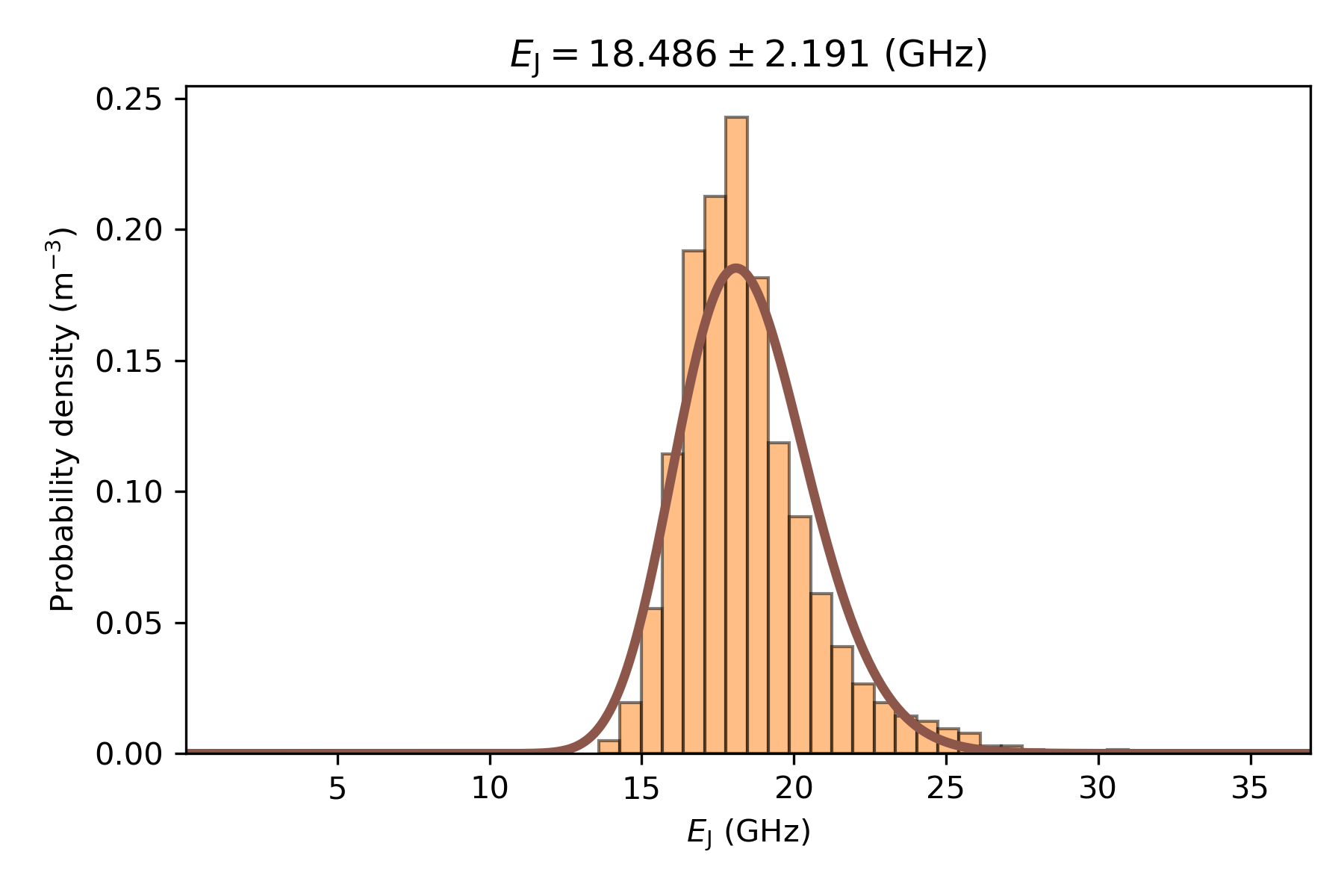
Fig. 1.5.26 Histogram of the distribution of Josephson energies for the 5000 samples simulated. A log-normal fit curve is also drawn. The mean \(E_\mathrm{J}\) and its standard deviation are displayed.
Some of the parameters for plot_distribution are
ghz: IfTrue, results are shown in GHz; otherwise, they are in joules.fit: IfTrue(default), a log-normal fit is shown alongside the distribution.output: Optional path to where save the figure.xlims: Controls x-axis limits.
Note
If we have used xlims="auto", the x-axis limits would be extended to cover the whole range of energies found. This is showcased in Fig. 1.5.27.
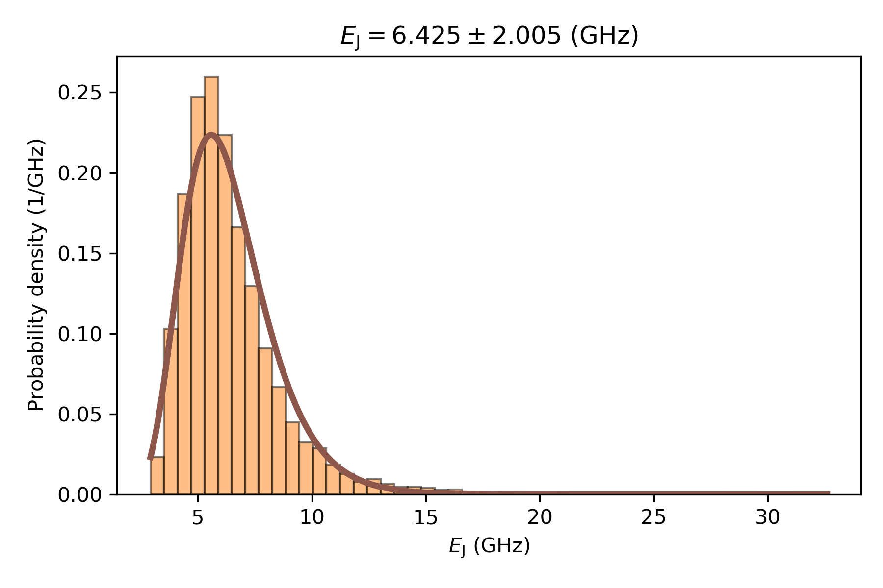
Fig. 1.5.27 Histogram of the distribution of Josephson energies for the 5000 samples
simulated.
Equivalent to Fig. 1.5.26, but
xlims="auto" was used, so the whole energy distribution is shown.
1.5.2. Plotting the rough interfaces
The plot_surfaces
method displays the height profiles of the two interfaces for a given junction
realization.
# Visualize the rough interfaces for the first realization (index 0).
surface_idx = 0
slv.plot_surfaces(
    idx=surface_idx, output=output_dir / f"interface_roughness-{surface_idx}.png"
)
Intensity plots showing the height profile of the two interfaces associated to the first junction of the sample is shown in Fig. 1.5.28.
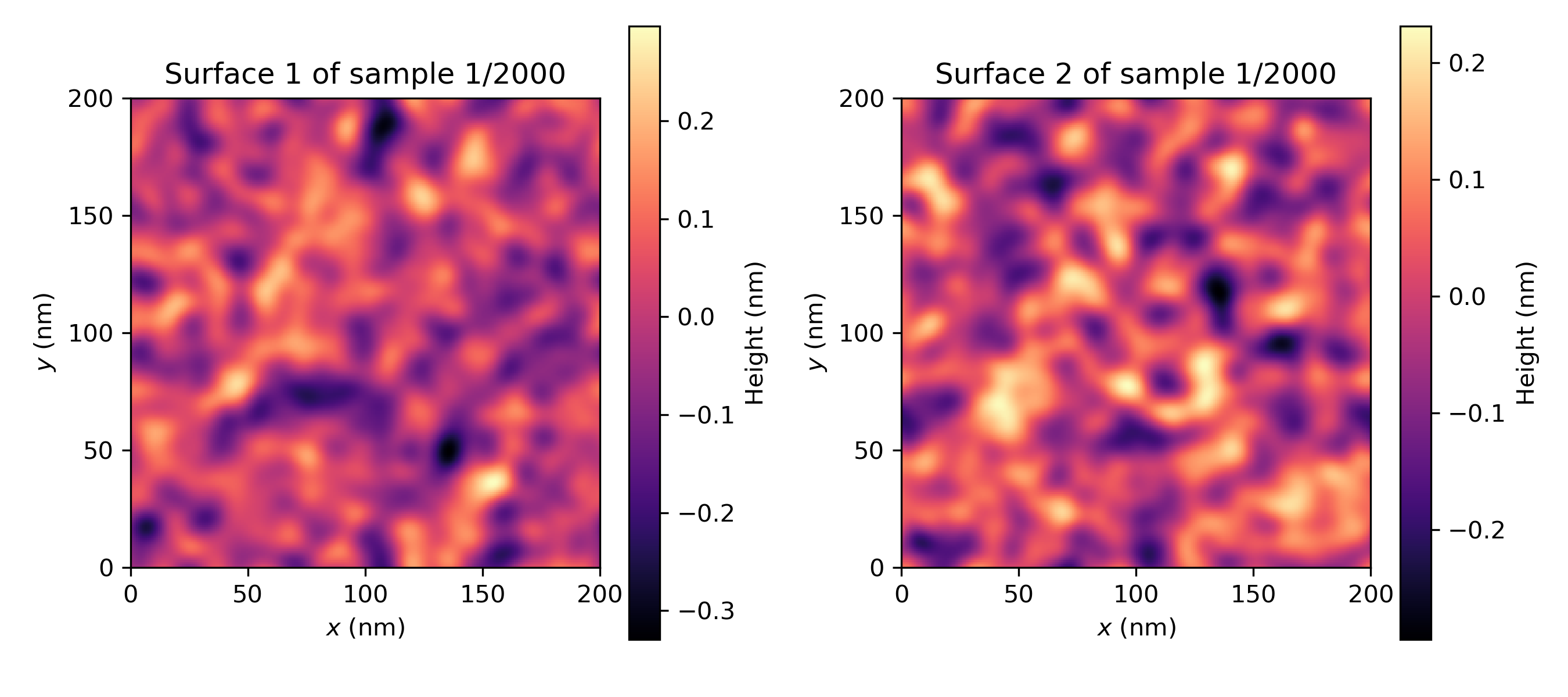
Fig. 1.5.28 Intensity plots of the height profile of the two Al/AlOx interfaces associated to the first Josephson junction simulated.
Some of the parameters for plot_surfaces include:
idx: The index of the junction realization to plot (from 0 ton_samples - 1).nm: IfTrue(default), height variations are shown in nanometres; otherwise, they are in meters.output: Optional path to where save the figure.
1.6. Full code
__copyright__ = "Copyright 2022-2026, Nanoacademic Technologies Inc."

"""
Analysis of Josephson-energy variability induced by interface roughness
"""
from pathlib import Path
from qtcad.transport.josephson_junction import GaussianRandomField, SolverParams, Solver
import qtcad.device.constants as ct

# Directories and file paths.
script_dir = Path(__file__).parent.resolve()
# Directory to store any output files.
output_dir = script_dir / "output" / "josephson_energy_variability"
output_dir.mkdir(parents=True, exist_ok=True)

# Set up the roughness model.
# · sigma: RMS height for (interface 1, interface 2) in metres.
# · ksi: transverse correlation length in metres.
sigma = (0.085e-9, 0.085e-9)
ksi = 25e-9
roughness_model = GaussianRandomField(sigma=sigma, ksi=ksi)

# Instantiate the solver parameters with default values.
params = SolverParams()

# Number of partitions along x and y.
params.n_partitions = (256, 256)

# Number of different junctions to sample.
params.n_samples = 5000

# Effective potential barrier height in joules.
params.potential_barrier_height = 1.1 * ct.e

# Seed for the random number generator to ensure reproducibility.
params.rng_seed = 3141592


# Nominal thickness of the AlOx layer.
thickness = 1e-9

# Side lengths of the junction.
side_lengths = (120e-9, 120e-9)

# Initialize the solver.
slv = Solver(
    solver_params=params,
    roughness_model=roughness_model,
    thickness=thickness,
    side_lengths=side_lengths,
)

# Run the simulation.
slv.solve()


# Show the statistical results for E_J.
ej_mean_ghz = slv.mean_value / (ct.h * 1e9)
ej_std_ghz = slv.std_deviation / (ct.h * 1e9)
print(f"Mean E_J: {ej_mean_ghz:.3f} GHz")
print(f"Standard deviation of E_J: {ej_std_ghz:.3f} GHz")

# Accessing the raw energy distribution for a custom analysis.
# raw_energies = slv.energy_distribution

# Plot the Josephson energy distribution with a fit curve.
slv.plot_distribution(ghz=True, fit=True, output=output_dir / "E_J_distribution.png")

# Visualize the rough interfaces for the first realization (index 0).
surface_idx = 0
slv.plot_surfaces(
    idx=surface_idx, output=output_dir / f"interface_roughness-{surface_idx}.png"
)