2. Automated Josephson-junction geometry extraction from layout

2.1. Requirements

2.1.1. Software components

QTCAD
KLayout (optional, for layout inspection)

2.1.2. Python script

qtcad/examples/tutorials/josephson_junction_variability_layout.py

2.1.3. Layout file

qtcad/examples/tutorials/layouts/jj_169nm_82nm.oas

2.1.4. References

Josephson-energy solver
Analysis of Josephson-energy variability induced by interface roughness
Zhu et al. [ZBG26]

2.2. Briefing

In this tutorial, we demonstrate how to perform a Josephson-energy variability analysis with an automatic extraction of the dimensions of a Josephson junction from a layout file (OASIS or GDS). Such an automated extraction ensures that the simulated geometry perfectly matches the intended device layout, bridging the gap between physical layout design (CAD) and numerical simulation.

We will mostly follow the setup of the tutorial Analysis of Josephson-energy variability induced by interface roughness. However, instead of defining a square junction manually, we will use a layout file that defines a junction with different side lengths. For a detailed discussion of the underlying theory and the Josephson-energy solver, please refer to Analysis of Josephson-energy variability induced by interface roughness and Zhu et al. [ZBG26].

2.3. Josephson-energy variability simulation

2.3.1. Imports and paths

We begin by importing the necessary modules from QTCAD^® and defining some paths.

"""
Josephson-energy variability: automated extraction of geometry parameters from layout
"""

from pathlib import Path
from qtcad.transport.josephson_junction import GaussianRandomField, SolverParams, Solver
import qtcad.device.constants as ct

# Directories and file paths.
script_dir = Path(__file__).parent.resolve()
layout_dir = script_dir / "layouts"
# Directory to store any output files.
output_dir = script_dir / "output" / "josephson_energy_variability"
output_dir.mkdir(parents=True, exist_ok=True)

Let us also define the path to the layout file associated with the desired Josephson junction layout. Fig. 2.3.5 shows the layout visualized using KLayout.

# Define the path to the OASIS layout file.
layout_path = layout_dir / "jj_169nm_82nm.oas"

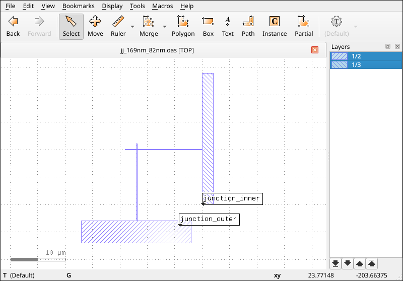
Fig. 2.3.5 Layout of a Josephson junction visualized in KLayout. The layout has two named overlapping shapes, `junction_inner` and `junction_outer`.

2.3.2. Roughness model and solver parameters

As in the previous tutorial, we set up our Gaussian-random-field model for the interface roughness and define the transport calculation parameters. We will use the same physical parameters, but note that the layout we are about to load defines a different junction. Here, we will deal with a rectangular junction with side lengths \(169\) and \(82\) nm, whereas the previous tutorial considered a square one with side length \(200\) nm.

For a detailed explanation of the parameters used below (such as sigma, ksi, n_partitions, and n_samples), please refer to the corresponding sections in Analysis of Josephson-energy variability induced by interface roughness or directly to the API reference of SolverParams.

# Set up the roughness model.
sigma = (0.085e-9, 0.085e-9)
ksi = 10e-9
roughness_model = GaussianRandomField(sigma=sigma, ksi=ksi)

# Instantiate the solver parameters.
params = SolverParams()
params.n_partitions = (512, 256)
params.n_samples = 2000
params.potential_barrier_height = 1.1 * ct.e
params.rng_seed = 3141592

2.4. Extracting geometry parameters from a layout file

QTCAD^® allows automated extraction of the geometry parameters of Josephson junctions from a layout file by identifying the rectangular overlap between the shapes forming the junction in an OASIS or GDS file.

2.4.1. Layout file requirements

For the automated extraction algorithm to succeed, the layout file provided must satisfy three conditions:

Exactly two named shapes: The file must contain exactly two shapes, and each shape must have an associated label that serves as its name. These labels allow the solver to distinguish the two superconducting leads.
Single rectangular overlap: The intersection of these two shapes must form a single rectangle. This rectangle will defines the active tunnelling area. SQUID designs are not supported.
Axis alignment: The resulting junction must be aligned along the \(x\) and \(y\) axes. Rotated junctions are not supported for automated side length extraction.

If any of these conditions are violated, the solver will raise a ValueError during initialization.

2.4.2. How to consider a junction layout file

Now, given a layout file defining a Josephson junction from two overlapping shapes, instead of passing side_lengths to the Solver, we only need to provide the path to the layout file via the layout_file parameter.

Note

When layout_file is used, side_lengths should not be passed

# Nominal thickness of the AlOx layer.
thickness = 1e-9

# Initialize the solver using the layout file.
# Note: `side_lengths` should not be passed when `layout_file` is used.
slv = Solver(
    solver_params=params,
    roughness_model=roughness_model,
    thickness=thickness,
    layout_file=layout_path
)

# Upon initialization, the solver parses the layout and calculates the side lengths.
l_x, l_y = slv.side_lengths
print(f"Automatically extracted side lengths: {l_x * 1e9:.1f} nm x {l_y * 1e9:.1f} nm")

Note that the extraction happens during instantiation. If the layout parsing is successful, the side_lengths attribute of the slv object is automatically set. Users can then optionally directly inspect the dimensions before starting the simulation, as done in this example:

Automatically extracted side lengths: 169.0 nm x 82.0 nm

Integration into electromagnetic simulation workflows

If you want to integrate the Josephson-energy solver into an electromagnetic-simulation workflow starting from the 2D layout of a superconducting chip, make sure to have two sets of layout files:

A layout file for each distinct Josephson-junction design. These will be used in the Josephson-energy solver, SolverParams.
One with the full chip layout, where the distributed junctions are replaced by rectangular inductive-port elements. The 3D geometry and mesh files generated from it will be used in QTCAD^® electromagnetic solvers. For instance, the capacitance or Maxwell eigenmode solvers.

2.5. Running the simulation and extracting results

Once the geometry is extracted, the rest of the workflow is identical to the case with direct input of the side lengths.

# Run the simulation.
slv.solve()

# Show the statistical results for E_J.
ej_mean_ghz = slv.mean_value / (ct.h * 1e9)
ej_std_ghz = slv.std_deviation / (ct.h * 1e9)
print(f"Mean E_J: {ej_mean_ghz:.3f} GHz")
print(f"Standard deviation of E_J: {ej_std_ghz:.3f} GHz")

The output will be similar to

Mean E_J: 6.384 GHz
Standard deviation of E_J: 1.143 GHz

2.5.1. Visualizing results

As shown in Analysis of Josephson-energy variability induced by interface roughness, we can easily visualize the distribution of results and the profile of the rough interfaces using plot_distribution and plot_surfaces, respectively.

# Plot the Josephson energy distribution with a fit curve.
slv.plot_distribution(
    ghz=True, fit=True, output=output_dir / "E_J_distribution_layout.png"
)

# Visualize the rough interfaces for the second realization (index 1).
surface_idx = 1
slv.plot_surfaces(
    idx=surface_idx, output=output_dir / f"interface_roughness-{surface_idx}.png"
)

The resulting plot of the energy distribution is shown in Fig. 2.5.11 and the intensity plots showing the interfaces’ height profile is shown in Fig. 2.5.12.

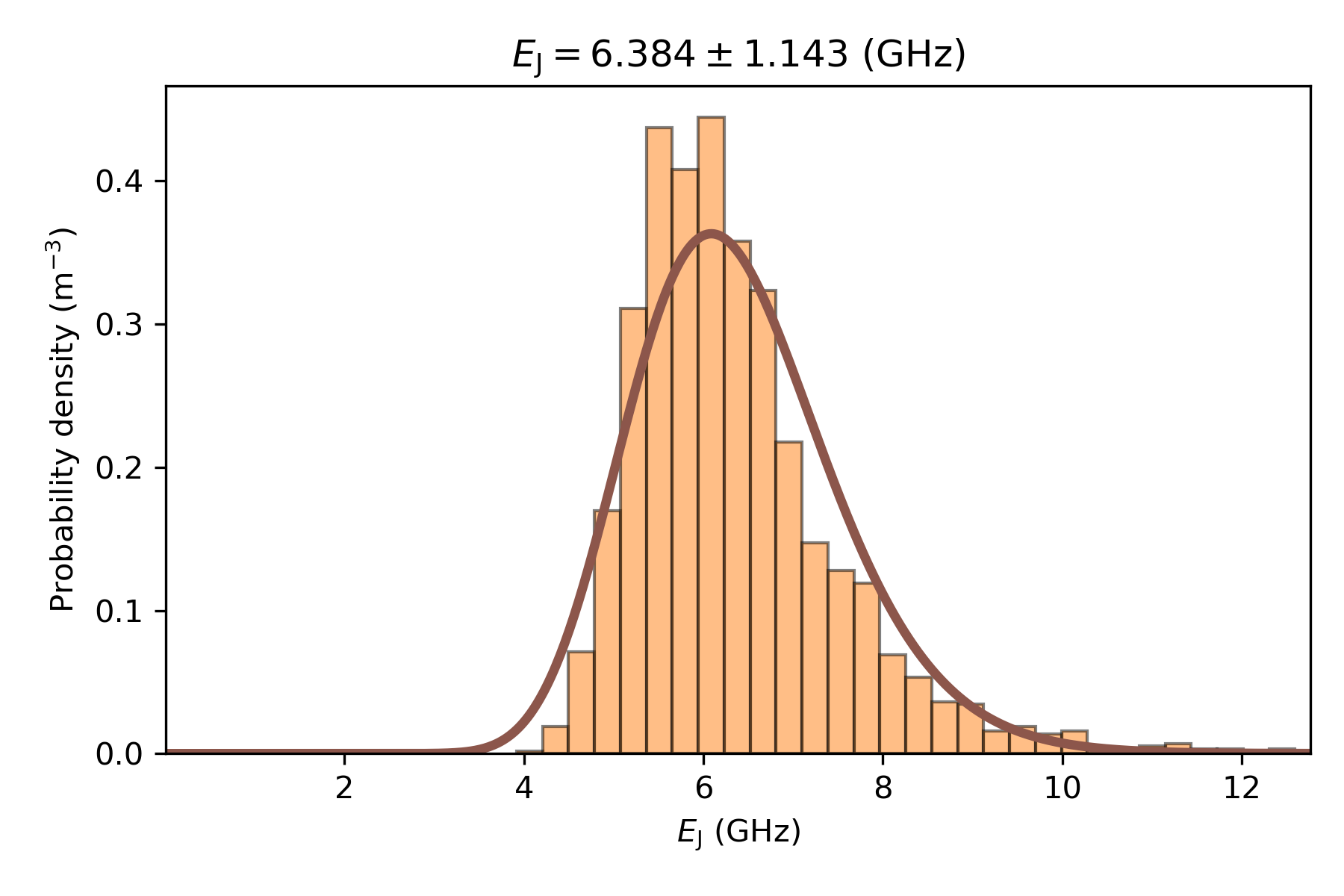
Distribution of the Josephson energy for 2000 samples. — Fig. 2.5.11 Histogram of the distribution of Josephson energies for the 2000 samples simulated. A log-normal fit curve is also drawn. The mean \(E_\mathrm{J}\) and its standard deviation are displayed.

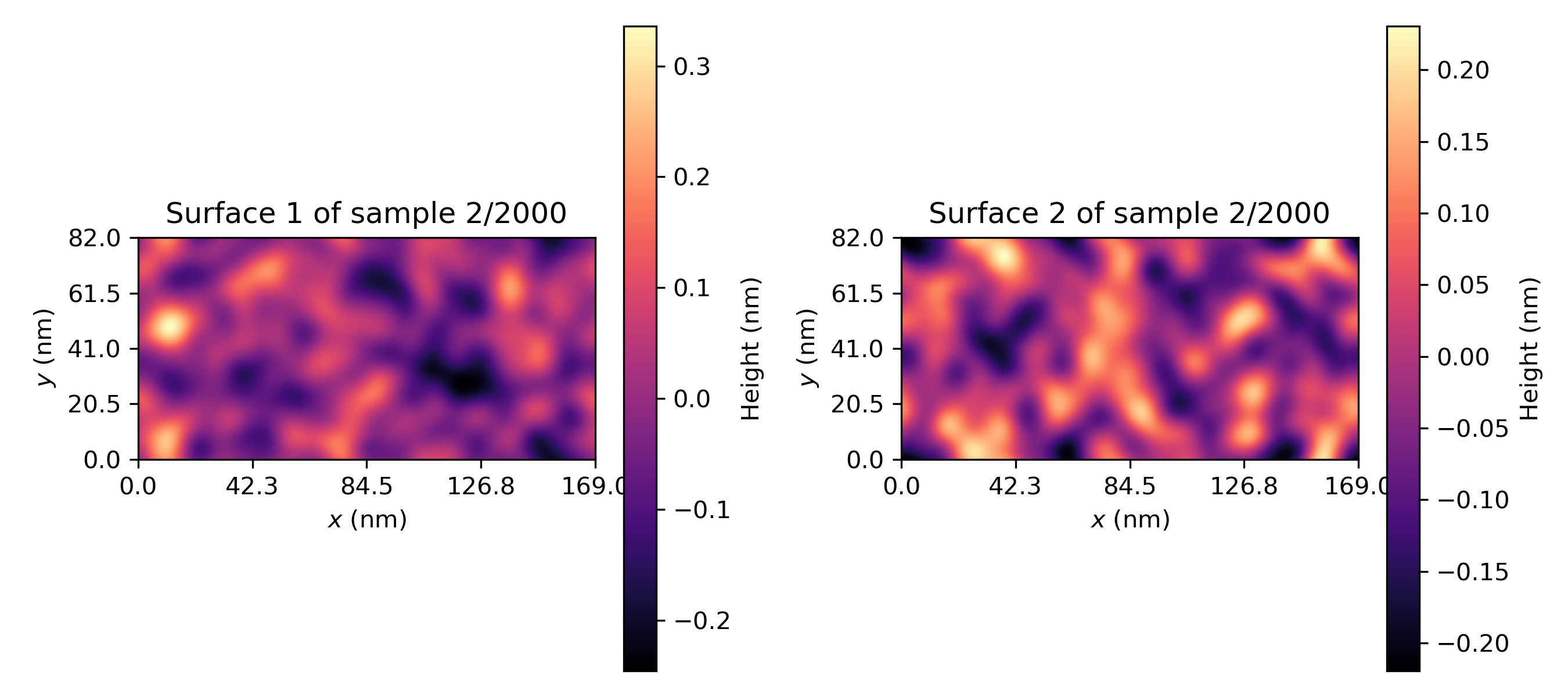
Height profiles of the two interfaces associated to the second junction. — Fig. 2.5.12 Intensity plots of the height profile of the two Al/AlO_x interfaces associated to the second Josephson junction simulated.

2.6. Full code

__copyright__ = "Copyright 2022-2026, Nanoacademic Technologies Inc."

"""
Josephson-energy variability: automated extraction of geometry parameters from layout
"""
from pathlib import Path
from qtcad.transport.josephson_junction import GaussianRandomField, SolverParams, Solver
import qtcad.device.constants as ct
# Directories and file paths.
script_dir = Path(__file__).parent.resolve()
layout_dir = script_dir / "layouts"
# Directory to store any output files.
output_dir = script_dir / "output" / "josephson_energy_variability"
output_dir.mkdir(parents=True, exist_ok=True)

# Define the path to the OASIS layout file.
layout_path = layout_dir / "jj_169nm_82nm.oas"

# Set up the roughness model.
sigma = (0.085e-9, 0.085e-9)
ksi = 10e-9
roughness_model = GaussianRandomField(sigma=sigma, ksi=ksi)

# Instantiate the solver parameters.
params = SolverParams()
params.n_partitions = (512, 256)
params.n_samples = 2000
params.potential_barrier_height = 1.1 * ct.e
params.rng_seed = 3141592

# Nominal thickness of the AlOx layer.
thickness = 1e-9

# Initialize the solver using the layout file.
# Note: `side_lengths` should not be passed when `layout_file` is used.
slv = Solver(
    solver_params=params,
    roughness_model=roughness_model,
    thickness=thickness,
    layout_file=layout_path
)

# Upon initialization, the solver parses the layout and calculates the side lengths.
l_x, l_y = slv.side_lengths
print(f"Automatically extracted side lengths: {l_x * 1e9:.1f} nm x {l_y * 1e9:.1f} nm")

# Run the simulation.
slv.solve()

# Show the statistical results for E_J.
ej_mean_ghz = slv.mean_value / (ct.h * 1e9)
ej_std_ghz = slv.std_deviation / (ct.h * 1e9)
print(f"Mean E_J: {ej_mean_ghz:.3f} GHz")
print(f"Standard deviation of E_J: {ej_std_ghz:.3f} GHz")


# Plot the Josephson energy distribution with a fit curve.
slv.plot_distribution(
    ghz=True, fit=True, output=output_dir / "E_J_distribution_layout.png"
)

# Visualize the rough interfaces for the second realization (index 1).
surface_idx = 1
slv.plot_surfaces(
    idx=surface_idx, output=output_dir / f"interface_roughness-{surface_idx}.png"
)